

In finite element modeling, you may encounter formulations where a force does not monotonically increase with displacement. You can see this property in many material models that include degradation of the material. Such behavior is represented by a negative stiffness. In this blog post, we discuss some examples of negative stiffness, including the physical backgrounds and numerical implications. These ideas are not confined to mechanical analysis, even though the term stiffness originates in that field.
An Example of Negative Stiffness
Let’s consider a symmetric two-bar structure under a compressive load, as shown in the following figure:
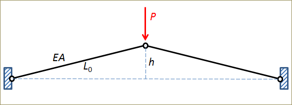
Two bars under compression.
We assume that the bars are linearly elastic so that the force in a bar, F, is
where Δ is the elongation and L0 is the original length.
Using Pythagoras’ theorem, the vertical force can then be written as an explicit function of the vertical displacement:
The following quantities have been nondimensionalized:
- The normalized displacement \delta = w/h, where w is the deflection under the load. Thus, \delta=1 when the bars are horizontal and \delta=2 when the structure is upside down.
- The parameter \kappa = h/L_0 is the aspect ratio: the initial height relative to initial bar length.
The force as a function of displacement is shown in the graph below. The example actually shows as a buckling problem with snap-through. Between points A and C, no unique solution exists. In a previous blog post, we further discuss the concept of buckling in structures.
The compressive force in the bars increases until they are horizontal (\delta=1), but the vertical projection decreases even faster beyond point A. This is why the vertical force decreases.
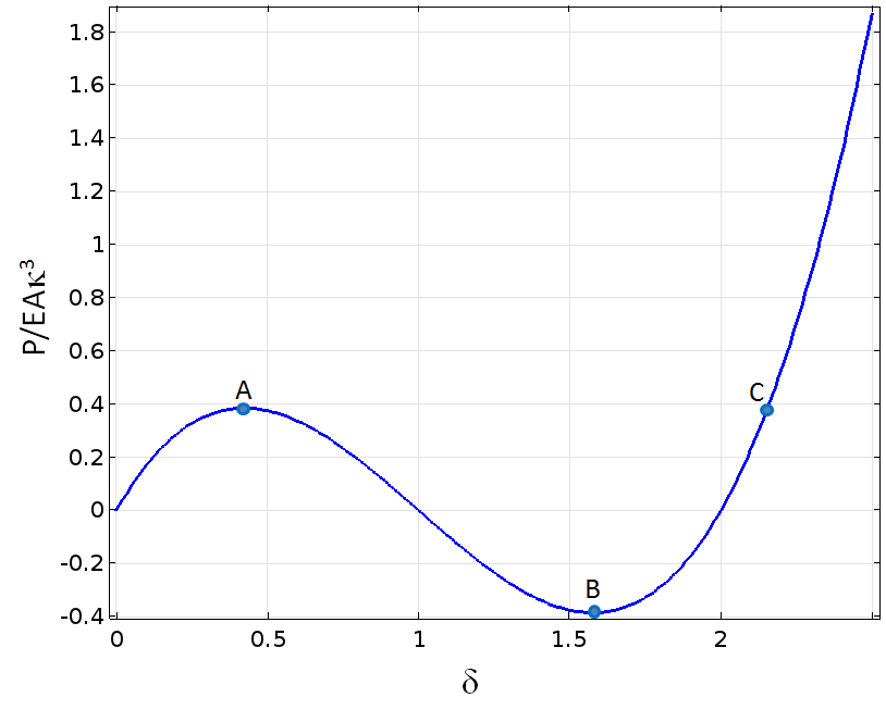
Force as a function of vertical displacement.
If we build a finite element model of this structure and try to increase the load, the analysis will probably fail when we reach the first peak at point A. We can, however, easily trace the solution by prescribing the vertical displacement at the loaded point, rather than the force. The applied force can then be obtained as the reaction force. The graph above was created using that method.
The tangential stiffness for this single degree of freedom system is defined as the rate of change in force with respect to displacement:
The stiffness is thus negative between points A and B. A negative stiffness is often related to numerical and physical instabilities.
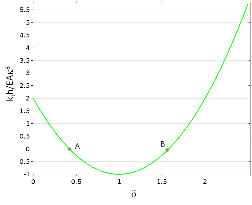
Stiffness as a function of vertical displacement.
Negative Stiffness in Softening Materials
There are several material models within the field of solid mechanics that contain a negative slope of the stress-strain curve, either as an intentional effect or with certain choices of parameters. For example, some models for concrete are designed like this. In the physical interpretation of this behavior, cracks form when the material model is loaded in tension. The load carried by a test specimen will then decrease. The cohesive zone models used for describing decohesion in the COMSOL Multiphysics® software also show this type of behavior.
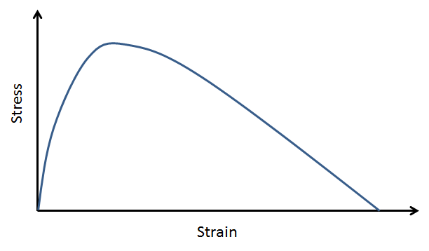
A strain-softening material.
At the material level, decreasing stress with increasing strain indicates a negative stiffness:
Such a material can only be tested under a condition of prescribed displacement; otherwise, it will fail immediately when the peak load is reached. The negative stiffness is thus related to a material instability.
In general, the stress and strain states are multiaxial. Stress and strain are represented by second-order tensors. In the multiaxial case, we must use a more general criterion for material stability: For any small change in the strain state, the corresponding change in the stress state must be such that the sum of the products of all stress and strain components is positive. That is,
Or, written in component form,
This is called Drucker’s stability criterion or Hill’s stability criterion.
The discretized form used in finite element analysis implies that the constitutive matrix relating stress increments to strain increments must be positive definite in order for the material to be stable. This is a condition that is generally computationally expensive to check for nonlinear materials. For a linear elastic material, the requirement can be directly converted into the well-known requirements E>0 and \quad -1< \nu < 0.5.
How can we mediate that we sometimes need to work with material models that do not fulfill the stability criterion? The important fact is that the material can be locally unstable, while the structure as such is still stable.
To understand this behavior, we can think of the material in the structure as connected springs. Some springs are purely elastic and represent the undamaged material, while a certain spring fails. Consider the three springs in the figure below.
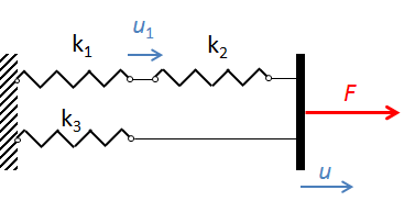
A three-spring system. The extension of the failing spring is denoted u1.
The spring k1 represents the material with the damage model, whereas the other two springs are purely elastic. The material model for the first spring is bilinear.
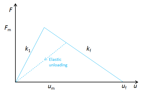
Material model for the nonlinear spring. The peak force Fm is reached at the displacement um.
The force in the lower branch is independent of damage:
Before the peak load is reached, the force in the upper branch is
since the two springs are connected in series.
The damage starts when the force in the upper branch is F_u = F_m; that is, when the external displacement is
and the corresponding external force is
During the degradation, the force in the damaged spring can be written as F_u = F_m-k_f \left(u_1-u_m \right). The same force also passes through spring 2 so that F_u = k_2(u-u_1).
These two relations determine u1 as a function of the external displacement:
In order to give a reasonable solution, u1 must increase when the external displacement is increased. Thus, it is necessary that k_2 > k_f. This is actually a clue to a very general result. A quick decrease in the force (or stress) is more susceptible to instability than a slower decrease.
Finally, we can derive the relation between the total external force and displacement during the degradation phase:
Thus, the external force can either increase or decrease when the external displacement increases, depending on the relative stiffness in the two branches. This simple model can thereby predict two types of instability:
- The upper branch can become unstable if k_2 > k_f
- Even if k_2 < k_f, the total system will be unstable if k_3 < \frac{k_2k_f}{k_2-k_f}
In either case, a slower decrease of the force in the damage model is beneficial. In other words, the stiffer the surroundings, the more plausible it is that the whole system will be stable.
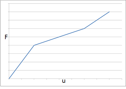
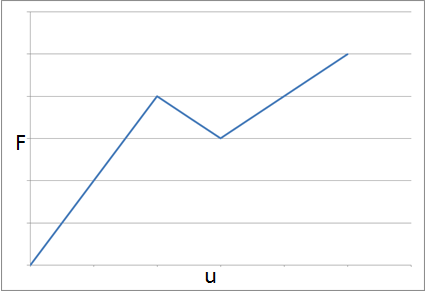
A globally stable system (left) and a system where the stiffness in the lower branch is too small to maintain stability (right).
In reality, we are not free to make arbitrary choices about force and stiffness. The area under the triangular force-displacement curve in the material model represents the energy dissipated by the process. The energy dissipation and the displacement (or strain) at final failure have a physical meaning.
An Energy Balance Interpretation
The damaged part of a structure elongates while its force decreases. If the external displacement remains fixed, then the elastic parts of the structure must contract to compensate. This means that elastic energy is released. The only way the energy can be absorbed is by doing work on the damaged part. If, for a certain incremental displacement \Delta u_1, the energy released by the elastic parts is larger than the work needed to produce the same displacement in the cracking part, the state is unstable.
Years ago, a friend of mine at the Department of Solid Mechanics at KTH Royal Institute of Technology in Stockholm performed some interesting experiments where he studied the stability of cracks in a ductile steel using extremely long three-point bend test specimens. The tests highlighted that crack stability is not only a function of the local stress state, but also of the capacity that the stored energy in the test specimen has to drive crack propagation. The longest test specimen in the experiments was 26 meters and occupied a large portion of the lab! The experiment was reported in the article “The stability of very long bend specimens” in the International Journal of Pressure Vessels and Piping.
Homogeneous Stress States
With softening material models, it is extremely difficult to achieve convergence in a finite element model if the stress state is homogeneous.
In a physical material, the strength does not have a perfectly uniform distribution. When increasing the load, a crack will form at the location with the lowest strength, even if the stress state is homogeneous. When this happens, the surrounding material is unloaded.
Consider this example of three elastic blocks joined by two glue layers:
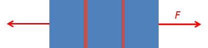
In real life, one glue layer will fail before the other. The slightly stronger layer will then be unloaded as the force through the part decreases. We cannot predict which layer will fail, since that is controlled by manufacturing inaccuracies. In the mathematical model, however, both layers fail simultaneously. Numerically, the iterations may not converge because the failure jumps back and forth between the two layers.
In a finite element model, the stresses are evaluated at each integration point within each element. When the load is increased above the maximum value, the failure may even jump between the elements or individual integration points within the same element (if the stress is the same everywhere).
This behavior implies that if we implement our own material model containing strain softening, we should test it using a single first-order element and under prescribed displacements. In this way, we ensure a homogeneous prescribed strain field and the stress is the same everywhere in the element. One example is Mazar’s damage model, which we described in a previous blog post. If we were to change the element shape functions to quadratic in that model, the analysis would no longer converge.
Does this mean that damage models are meaningless? Not at all. However, we must be careful to avoid indeterminate states. If a structure and its boundary conditions are symmetric, that symmetry must be employed in order to avoid indeterminacy. We can often solve problems with axial symmetry by using an axially symmetric model, while this may be impossible using a model of a 3D solid sector. Another approach is to allow a slight random spatial disturbance of the material data. This approach actually mimics nature, where strength values are randomly distributed. Also, it is important to increase the loading slowly in order to avoid large portions of the structure switching to a failed state at the same time.
Shear Bands
In some material models, for example, within soil plasticity, strongly mesh-dependent thin layers with high shear strains can occur. These layers are called shear bands. When yielding is first initiated, the surrounding elements or even integration points are unloaded. The first elements to yield continue to accumulate plastic strains. It is interesting that this type of instability can actually be seen in real soil and is not only an artifact in the numerical model. Just as in nature, we cannot predict the exact location and distribution of the shear bands in the model.
Overcoming Instabilities in COMSOL Multiphysics®
As mentioned in the initial example, using prescribed displacements rather than prescribed forces is a good way to stabilize the numerical problem. However, this approach is essentially limited to the following cases:
- A single point load can be replaced with a prescribed displacement.
- The strain state is homogeneous, as when performing single-element tests of a material model, so that the displacement is the same over an entire boundary.
- The instability can be controlled by the external boundary conditions. In the spring device discussed above, a global instability caused by too small of a value of k3 could be cured by using a prescribed displacement, but not an instability within the upper branch.
There is a more general method, which we can use to continue solving past a point of instability. In this method, we first define an arbitrary quantity that is known to monotonically increase and then add an extra equation that solves for the corresponding value of the prescribed load or displacement.
To display this technique, let’s augment the initial example with a spring, so that the load is applied by prescribing the deformation of the end of the spring. If the spring is very stiff, this is essentially the same as prescribing the displacement directly.
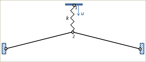
Bar system loaded through a spring.
If the spring is softer, the system may become unstable, since too much energy can be released by the spring. The critical value is
This is the most “negative stiffness” of the bar assembly, which occurs when the bars are horizontal. The relation between force and displacement at point 1 when varying the spring stiffness is shown below. The spring stiffness is given as
where the coefficient β is varied from an essentially stiff spring to values below the critical value.
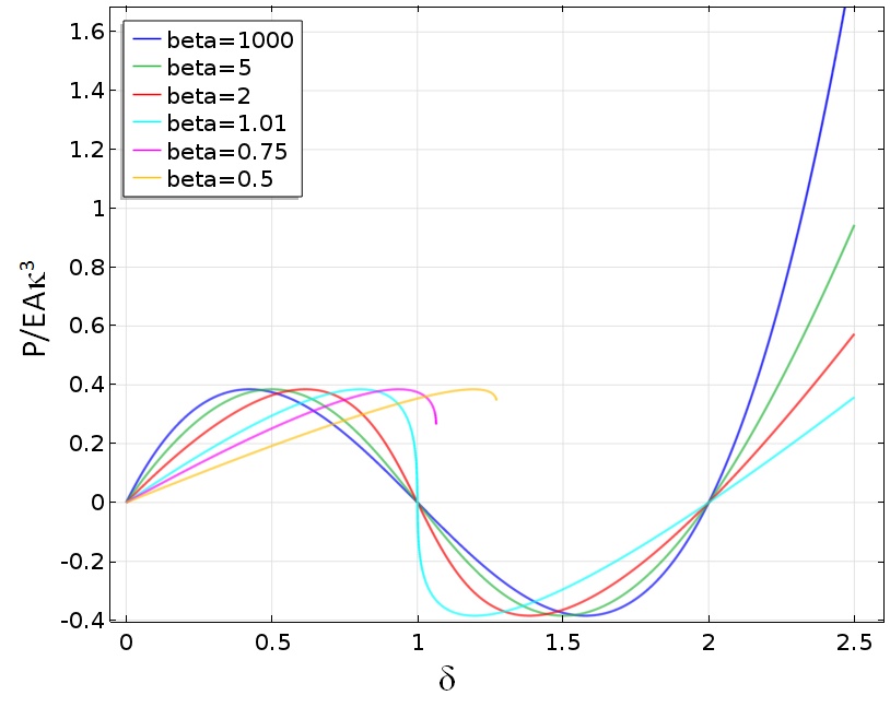
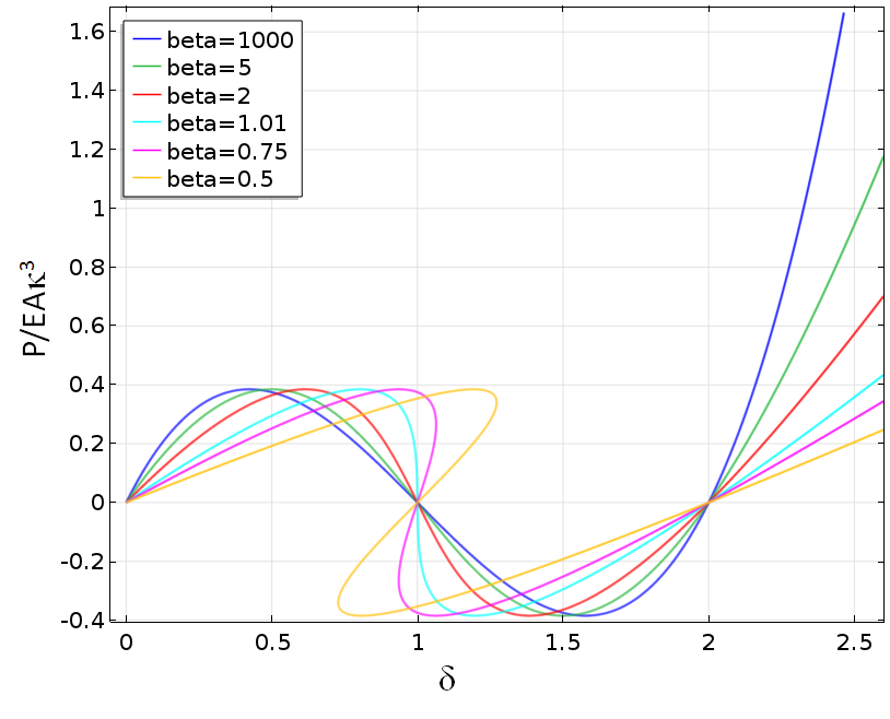
Force as a function of the displacement at point 1 when varying the spring stiffness.
For values of β smaller than one, the solution fails when the spring stiffness equals the “negative” stiffness of the bar assembly.
If a prescribed force is used instead, all solutions will fail at the first peak load. By using prescribed displacement, it is possible to continue the analysis further. For lower spring stiffness values, we are still limited by the state when the internal instability causes failure.
The solution that we want to track has a monotonic vertical displacement at point 2, but prescribing it directly is not possible, since this would change the problem fundamentally. Instead, we add an equation stating: “Set the spring end displacement at point 1 so that the monitored displacement at point 2 has the specified value.” To do this, we add a Global Equation node in which a new unknown variable disp_at_P1 is added.
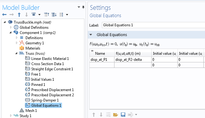
The Global Variable definition.
The equation determining the value of disp_at_P1 states that disp_at_P2-delta = 0. The variable delta is the monotonic parameter incremented in the Stationary study step and disp_at_P2 is a variable that contains the current value of the displacement at point 2.
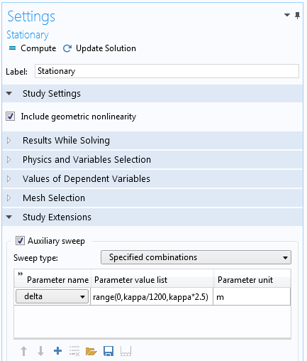
Settings for the study step, where delta is used as the auxiliary sweep parameter.
After solving, the displacement at point 2 will match the list of values of delta as specified in the Auxiliary sweep.
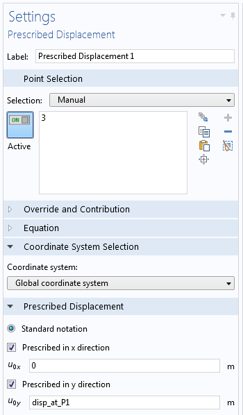
Settings for the prescribed displacement at point 1.
With this modification, it is possible to trace the solution through the instability. As seen in the following graph, even strong instabilities can be bypassed using this method.
Force as a function of the displacement at point 1 when varying the spring stiffness after stabilization with a Global Equation node.
Further Resources
- Browse these Application Gallery examples to learn more about modeling negative stiffness and instabilities in structures:
- S. Kaiser, “The stability of very long bend specimens”, Int. J. Pres. Ves, & Piping. 17 (1984) 1–17.


Comments (3)
Ivar Kjelberg
December 6, 2016Thank you Henrik, for a very nice Blog with useful “tricks” how to handle highly non-linear behavior with COMSOL.
Indeed, Negative Stiffness, and controlled Buckling as such, are interesting phenomena, we have been using them for years in our flexure design for snap in mechanisms, and very low stiffness solutions in flexure based metrology solutions.
Our colleague, now professor at the EPFL, Simon Henein has summarized some of these effects here https://infoscience.epfl.ch/record/186861/files/Flexure_delicaces_ms-3-1-2012_published.pdf .
And other companies such as MinusK.com and others here in Europe have used it for vibration isolation systems.
Yu Zhang
April 23, 2018Hi, Henrik:
Thank you for sharing us this useful technique to deal with softening processes. Now, I encountered a convergence issue caused by the stiffness degradation. In my model, when the tensile stress reaches a certain value, the damage initiates, and then the Young’s modulus degrades correspondingly. This would cause the convergence issue. I am trying to use your method, but it seems more complicated for my case because the load in my case is the the pore pressure which is not able to transform to a displacement load. Could you please share me a basic idea to solve this convergence issues. Any help would be highly appreciated.
Yu
Henrik Sönnerlind
April 24, 2018Hi Yu,
It is difficult to tell. One problem which often occurs with deteriorating materials is that all damage is localized to certain unstable points (the shear band problem, discussed above). The best way of dealing with that is probably to add some regularization.
Such techniques are discussed in this COMSOL Conference paper by Tobias Gasch:
https://www.comsol.com/paper/download/357911/gasch_paper.pdf
Regards,
Henrik