
You can easily include a PID controller in your simulations in the COMSOL Multiphysics® software. The PID Controller add-in, available as of version 5.5, can be added to any simulation project. It implements a standard proportional integral derivative (PID) controller with additional functionality, such as integral anti-windup and filtering of the derivative part. Such controllers are widely used in industrial process control. Here, we describe how to use the PID controller and show it in action with two simulation examples.
Introducing the PID Controller Add-In
Add-in functionality was made available as of COMSOL® version 5.5. An add-in is a combination of custom Settings windows and model methods that form some general functionality that users can add to any simulation model.
The PID Controller add-in is one of the example add-ins included with COMSOL Multiphysics and is available from the Add-in Libraries window, which you open from the Developer toolbar. When you have imported the PID Controller add-in, you can then add it to your model from the Add-ins menu (also on the Developer toolbar). It then appears as a PID Controller node under Global Definitions in the Model Builder. The figure below shows the Settings window for the PID Controller:
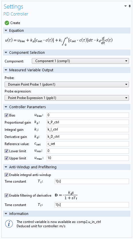
The Settings window for the PID Controller add-in. In the Information section, you find information about the created control variable and its deduced unit.
PID Controller Equation
The equation for the PID controller is the standard implementation with an added optional bias for the control variable (output) u. For the derivative term, the setpoint (reference value) is not included, because the setpoint is usually constant with abrupt changes. Therefore, the setpoint does not contribute to the derivative term, other than as unwanted drastic outputs when changed.
Measured Value Output
For the measured value output (which appears as c(t) in the equation), you typically add a domain point probe, which models a measurement performed for the quantity that you want to control, such as temperature or species concentration. The domain point probe is added somewhere in the geometry as the controller feedback for the process that you want to control.
Controller Parameters
In the Controller Parameters section, you enter the PID parameters and the reference value (setpoint). In addition, you can add an optional bias to the control variable and limits to the output. In reality, there are almost always lower and upper limits for the actuator (a valve or heater, for example) that receive the output from the controller.
Under Anti-Windup and Prefiltering, you can include two common and useful additions to the PID controller:
- Integral anti-windup
- Filtering of the derivative part
The integral anti-windup is an addition to the PID algorithm that takes into account that actuators have limits. It can then happen that the control variable reaches the actuator limits, which effectively breaks the feedback loop, because the actuator remains at its limits. If there is an integral part in the controller, the error will then continue to be integrated and can become very large (that is, it “winds up”). This unwanted behavior can result in large transients in the case that the actuator saturates.
The integral part of the controller is essential for eliminating steady-state errors and can therefore normally not be turned off. The integral anti-windup addition is intended to avoid the windup by an extra feedback loop with an error signal defined as the difference between the control variable and the actuator output. It means that the error is zero when the actuator does not saturate. When the actuator saturates, however, the anti-windup algorithm will attempt to drive the integrator to a value that makes the controller output be at exactly the saturation limit, preventing the windup. The rate of this reset is determined by the feedback gain 1/T_t, where T_t is the time constant that you can enter in the Settings window for the PID Controller add-in. The smaller the time constant, the faster the integral is reset.
The filtering of derivative is a low-pass filter for the derivative part of a PID controller. A problem with the derivative part is that it’s sensitive to noise. In many cases, the derivative part is not used, and the controller becomes a PI controller. With the filtering of the derivative part active, that part becomes more useful because high-frequency noise in the measurement will be removed and it will act as a derivative of low-frequency parts of the feedback signals. The parameter T_f is the time constant that you can enter in the Settings window for the PID Controller add-in to control the amount of filtering. The larger the time constant, the more filtering is applied to the derivative term.
Creating the Controller and the Information Section
When you have set up your PID controller, click the Create button at the top of the Settings window. It then creates a 0D component that contains the PID controller implemented as global equations. In the Information section, you see the name of the created control variable, such as comp2.u_in_ctrl. That is the variable that you enter where the control variable should act, such as an inflow velocity or a heat source that affects the measured value that you want to control.
The Information section also shows the deduced unit for the controller, which should match the unit of the acting quantity in the model (for example, m/s for a velocity or W for a heat source). If the units for the controller parameters are inconsistent, there is a message about the unit inconsistency in the Information section, and no PID controller is created.
Using Global Parameters
It is good practice to define the control parameters as global parameters. You can then vary them directly or through a parametric sweep to evaluate the controller’s performance and tune its parameters. Otherwise, if you change the values of the controller parameters directly in the PID Controller add-in, you need to create a new controller each time.
In the following sections, we will look at two examples of using the PID Controller add-in.
Controlling the Species Concentration in a CFD Model
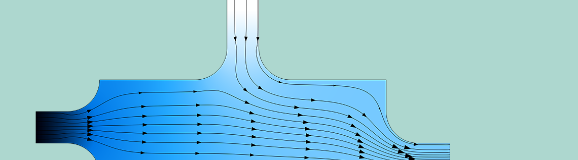
The Process Control Using a PID Controller model is available in the Application Library for COMSOL Multiphysics, with the PID controller implemented as a user-defined global equation. In this example, an inflow is used to control the oxygen concentration at the ignition point in a combustion chamber. The measurement of the oxygen concentration is implemented as a Domain Point Probe feature.
You can now download an updated version of this model using the Application Library update. In the updated version, the PID controller is instead created using the PID Controller add-in, using the settings as shown in the screenshot above. The PID parameters and the setpoint are defined as global parameters. Note that the PID parameters have negative values, which reflects that the controller action is reversed: It controls the speed of the inflow of a flow with a low oxygen concentration that lowers the concentration at the ignition point.
This model example uses a parametric sweep to simulate the PID control with two different parameter values for the P part (the proportional gain). A probe plot shows the time evolution of the concentration and its time derivative during the simulation. When the simulation has finished, a plot shows the concentration for both values of the P parameter. Clearly, the higher proportional gain is beneficial, but when you keep increasing it further, the overshoot will start to increase. The integral part ensures that there is no steady-state error.
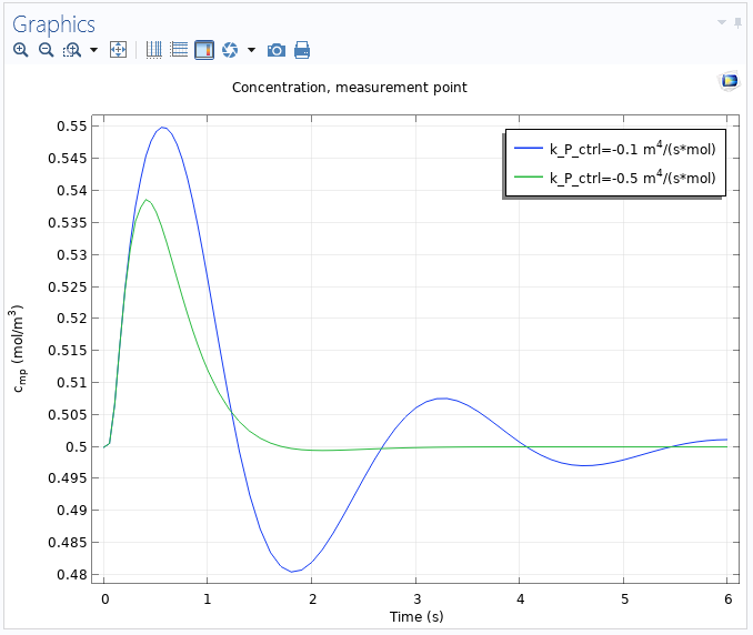
The concentration at the measurement point as a function of time for two values of the proportional gain k_P_ctrl.
Controlling Temperature in a Heating Model
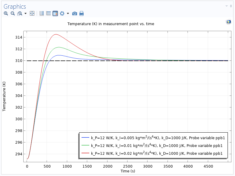
As a second example, consider a simple heat transfer model where a copper plate, surrounded by a material with a smaller thermal conductivity, is heated and the PID controller acts as a heat rate to control the temperature at a point outside the heater. The setpoint for the temperature is 310 K, and the entire plate is initially kept at room temperature, 293.15 K. There is a convective heat flux from all exterior boundaries with a heat transfer coefficient set to 5 W/(m^2 \cdot K). In the first simulation, all three PID parameters are varied in a parametric sweep to see their effect. The following plot shows the measured temperature versus time for a PI control only (the derivative gain is set to 0):
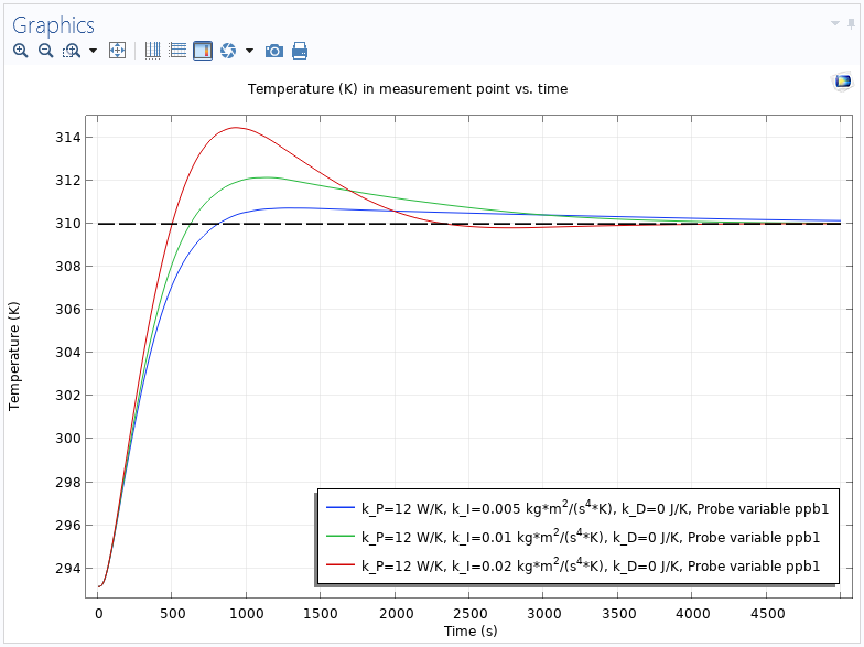
The temperature versus time for three different values of the integral gain and no derivative part. The dotted line indicates the setpoint (310 K).
The PID controller with the highest integral gain (the red curve) reaches the setpoint fastest, but at the expense of a larger overshoot. In the next plot, a derivative gain has been added so that a complete PID controller is used:
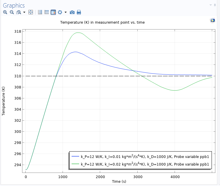
The temperature versus time for three different values of the integral gain and a derivative part, which speeds up the control.
As expected, the derivative gain reduces the settling time, making the PID controller faster than the PI controller.
Integral Anti-Windup to the Rescue
In a final simulation, the maximum heat rate is reduced to 100 W, which puts a limit on the control action. That limitation will cause integral windup for a PID controller, which is an effect that will degrade the controller performance. With this limitation, the lowest integral gain makes the controller response too sluggish, so in the following plots, the simulations with the two higher integral gains are included. The plot below shows the PID controller for the case when the integral anti-windup is turned off:
The temperature versus time when the heat rate is limited and the integral anti-windup is turned off. Due to the windup, large overshoots occur.
In the following plot, the integral anti-windup has been turned on, and it makes a dramatic change. There is now a smooth controller action, bringing the temperature to the desired setpoint with no or a very small overshoot. The higher integral gain can be used to make the controller faster without any adverse effects.
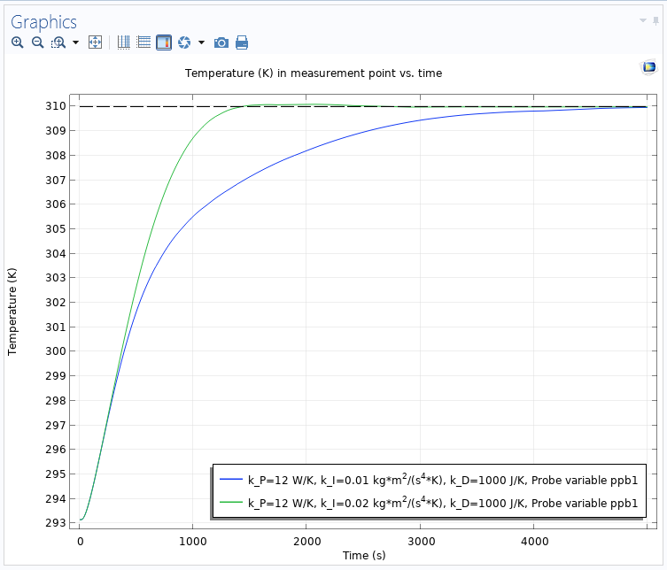
The temperature versus time when the heat rate is limited and the integral anti-windup is turned on, providing a smooth controller action without overshoots.
Next Steps
If you are interested in simulating the effect of a PID controller, try the PID Controller add-in that is available in COMSOL Multiphysics version 5.5. In addition, take a look at these resources:
- Try the Process Control Using a PID Controller tutorial model
- Read these related blog posts:


Comments (4)
Ivar KJELBERG
January 13, 2020Hi Magnus,
Nice Blog, and nice model to study, but …
PID is a bit simple and old fashioned today for precision controlled mechanisms, there are much better:
How about an example of an electromagnetic force actuated mechanism example, simplified as a force against a double mechanical mass-damper-springs model with a state space controller, with the state space matrix extracted from the COMSOL model of the mechanical system alone ?
I believe you have everything in COMSOL v5.5 now, but I’m still missing a first example to help us understand and train the state space extraction set-up of a more complex structural or lumped model, i.e. by defining action and metrology Points/BCs and getting the correct matrix, scaled at best.
Anyhow thanks for the present Blog already 🙂
Sincerely
Ivar
Magnus Ringh
January 14, 2020 COMSOL EmployeeHi Ivar,
Thanks! It’s been many years since I worked with industrial process control, but I think that PID controllers are still workhorses in many process control systems because of their ease of use and established tuning methods. That said, there are other interesting controller types that have their merits, and that includes state-space methods. We’ll see what we can do regarding examples of such controllers in future versions of COMSOL Multiphysics.
Best regards,
Magnus Ringh, COMSOL
Helger van Halewijn
January 23, 2020This example is a nice example of the evolution of Comsol. I have applied PID controllers to sensor models in measuring environmental pollution in air. Especially sensors to be used in cars and cities to monitor the quality of the air. The new development of the add-ins within Comsol is a step foreward and I am going to implement this for future use. Thanks for the clear explanation.
Regards,
Helger van Halewijn,
Helger van Halewijn
January 23, 2020q