Acoustics Module Updates
COMSOL Multiphysics® version 5.3 introduces new Acoustics Module functionality that greatly improves time-domain simulations of acoustics phenomena and facilitates solving large acoustics-based models. Further improvements include an array of new physics features and options as well as new postprocessing tools.
Overview of the Acoustics Module News
In summary, improvements to time-domain simulations include:
- Perfectly matched layers (PMLs) for pressure acoustics in the time domain
- The Thermoviscous Acoustics, Transient interface for the time domain
- Transient solver settings being controlled at the physics level for more robust simulations
- Speedup to the discontinuous Galerkin (dG) method
Large models benefit from the following new features:
- Ready-to-use suggested solver options for iterative solvers
- The option to use serendipity elements
New physics features and options include:
- New and improved stabilization techniques for linearized Navier-Stokes analyses that are based on the Galerkin least squares (GLS) method
- Improved formulation for the Slip boundary condition in Wall features for linearized Navier-Stokes and thermoviscous acoustics applications; this works very efficiently when using iterative solvers
- 2D axisymmetric formulation in the Convected Wave Equation interface
- Biot-Allard model to include thermal and viscous losses in poroelastic wave simulations
- New interior Perforated plate condition
- Improved ray acoustics formulation in 2D axisymmetric geometries
- Beam width calculations for far-field plots
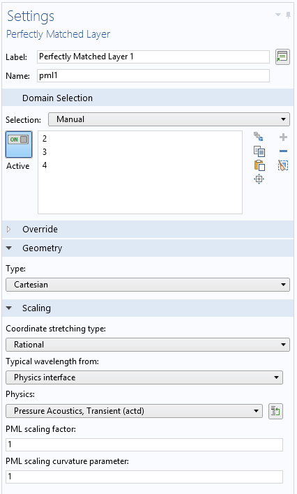
Perfectly Matched Layers for the Pressure Acoustics, Transient Interface
PMLs are often used in situations where the default first-order, nonreflective boundary conditions would generate spurious and unwanted numerical reflections. PMLs enable you to truncate the computational domain with an external layer that mimics waves moving into an infinite domain.
With COMSOL Multiphysics® version 5.3, the Pressure Acoustics, Transient physics interface now includes PML functionality in the time domain, for transient acoustic simulations based on the finite element method. This was previously only available for the Pressure Acoustics, Frequency Domain and Convected Wave Equation, Time Explicit interfaces. PMLs can be added from the Definitions node and support both polynomial and rational scaling options for 3D, 2D asymmetric, 2D, and 1D models in Cartesian, Cylindrical, and Spherical geometries.
Application Library path for an example that uses a PML in a time-dependent pressure acoustics simulation:
Acoustics_Module/Tutorials/gaussian_pulse_perfectly_matched_layers
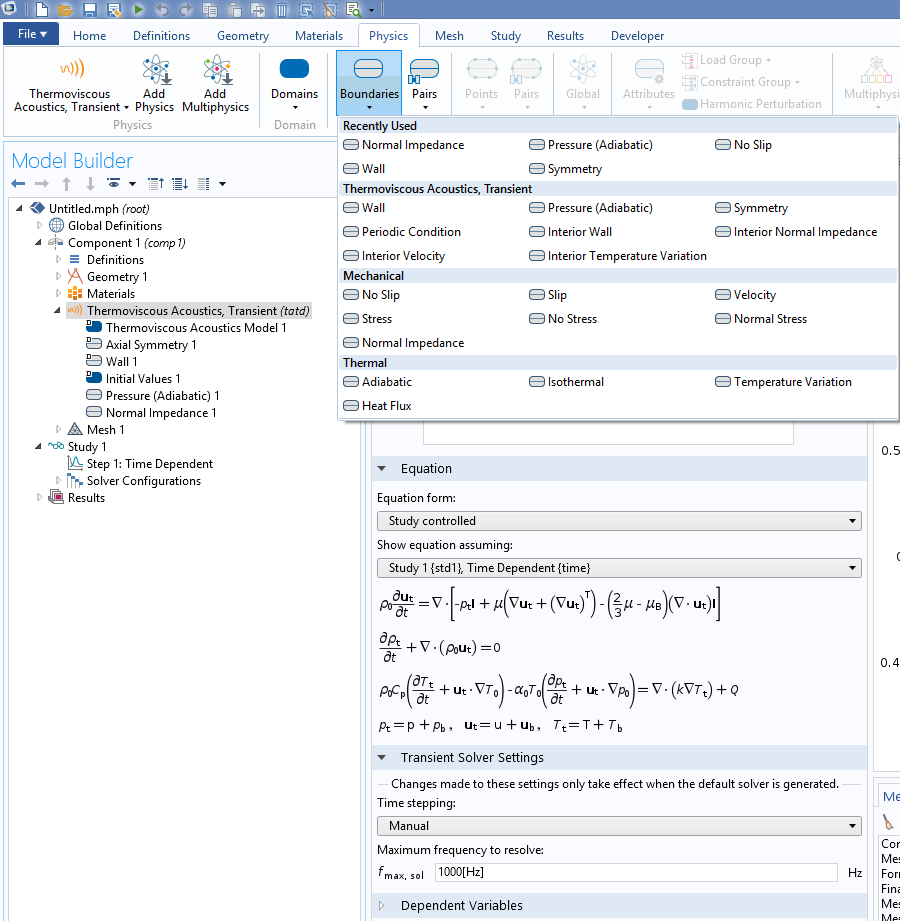
New Thermoviscous Acoustics, Transient Interface
The Thermoviscous Acoustics node has been extended to include an interface for time-dependent linear thermoviscous acoustics simulations, which includes source terms represented by any time-varying signal, such as Gaussian pulses. The Thermoviscous Acoustics, Transient interface is suited for modeling time-dependent wave propagation in systems where thermal and viscous losses are important — typically in applications with small dimensions like mobile devices, miniature loudspeakers, microphones, or in the holes of a perforate.
The interface can be coupled through the Thermoviscous Acoustic-Structure Boundary multiphysics interface to structural mechanics applications and interfaces such as Solid Mechanics, Shells, and Membranes.
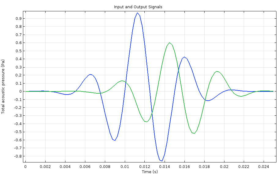 A COMSOL plot of the input and output signals.
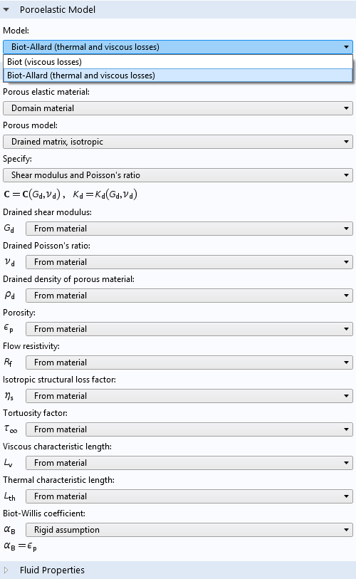
Poroelastic Waves Interface Updated with the New Biot-Allard Model
In applications where pressure and elastic waves propagate in porous materials filled with air, both thermal and viscous losses are important. A few example applications are insulation materials for room acoustics, lining materials in car cabins, foams used in headsets and speakers, and porous materials in mufflers.
To better simulate these types of applications, a Biot-Allard model option has been added to the Poroelastic Waves interface. Including this model supplements the previously available Biot model option, which considers only viscous losses and is useful for acoustic poroelastic wave propagation in rocks and soils where the saturating fluid is a liquid.
Up until now, the Pressure Acoustics, Frequency Domain interface together with an appropriate fluid model, such as the poroacoustic model, has been an adequate method for simulating many audio applications. However, these models do not capture all of the real-world effects and sometimes it is necessary to include elastic waves where, for example, the porous matrix needs to be coupled to vibrating structures. These can now be simulated with the new Biot-Allard model option in the Poroelastic Waves interface. Here, material inputs comply with typical conditions used and measured in audio and noise control applications.
Application Gallery link for an example using the Biot-Allard model option in a poroelastic wave simulation:
Multilayered Porous Material: Poroelastic Waves with Thermal and Viscous Losses (Biot-Allard Model)
Updated Acoustic-Structure Interaction Multiphysics Couplings
With the addition of the Biot-Allard model option to the Poroelastic Waves interface, multiphysics interfaces that couple poroelastic domains, structures, and acoustics have been revamped and improved. These support coupling pressure acoustics to poroelastic waves and poroelastic waves to structures (and sometimes all three). You can add a new interface using the Add Physics button in the ribbon, which opens the Add Physics window. The following updated Poroelastic Waves interfaces can be selected from the Acoustics and then Acoustic-Structure Interaction branches:
- Poroelastic Waves, a single-physics interface
- Acoustic-Poroelastic Waves Interaction, a multiphysics interface that adds the following physics and couplings:
- Pressure Acoustics, Frequency Domain
- Poroelastic Waves
- Multiphysics
- Acoustic-Porous Boundary
- Acoustic-Solid-Poroelastic Waves Interaction, a multiphysics interface that adds the following physics and couplings:
- Pressure Acoustics, Frequency Domain
- Solid Mechanics
- Poroelastic Waves
- Multiphysics
- Acoustic-Structure Boundary
- Porous-Structure Boundary
- Acoustic-Porous Boundary
- Solid Mechanics (Elastic Waves), an interface that adds the Solid Mechanics interface to the branch, effectively acting as a convenient shortcut to adding this interface from the acoustics location
2D Axisymmetric Formulation for the Convected Wave Equation, Time Explicit Interface
The Convected Wave Equation, Time Explicit interface is now available for use in 2D axisymmetric simulations. This extends the capabilities to model the propagation of acoustic waves over long distances, as a measure of the number of wavelengths. The interface features an Include out-of-plane components option that can be used to include out-of-plane components of a background flow and their interaction with the acoustic signal. This can be used, for example, to model axially symmetric ultrasound transducers or tweeters.
Predefined Iterative Solver Suggestions
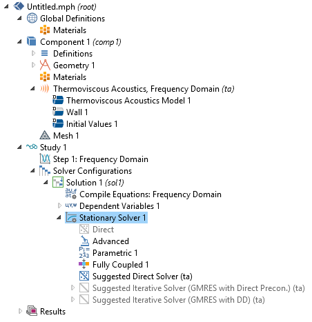
Several of the physics interfaces in the Acoustics Module now provide suggestions for alternate iterative solvers in addition to the default direct solver that is set up when the physics interfaces have been chosen and the model is solved for the first time. For some physics, two suggestions are given (as seen in the screenshot), where one solver is typically fast and the other more robust, but slower. The suggested solvers can be enabled when the direct solver runs into memory limitations and fails to converge. This new functionality simplifies the workflow when solving large models and does not require manual setup and tuning of iterative solvers when it has become apparent that the direct solver is not the optimal one to use.
Control of the Transient Solver from the Physics Nodes
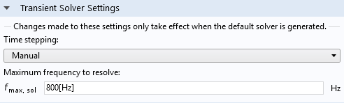
All the transient interfaces in the Acoustics Module now have a Transient Solver Settings section in the respective physics interface nodes. This sets up automatic controls of the default solver based on inputs provided in the new section, which leads to a better transient solver configuration and more robust simulations.
The default (and recommended setting) is to use the Manual option for the Time stepping drop-down menu and then enter the Maximum frequency to resolve in the appropriate edit field. In most acoustic problems, the frequency content of all sources is known or it can be evaluated by plotting the Fourier transform of the source signal. In linear acoustic applications, the sought-after solution will have the same frequency content as the source. Simply enter the frequency that you want to resolve in the new edit field. For nonlinear problems, a decision can be made on how many generated harmonics to resolve. In this case, the Maximum frequency to resolve edit field should be set to the number of harmonics multiplied by the source signal frequency.
Speedup of the Discontinuous Galerkin Method
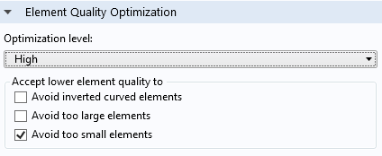
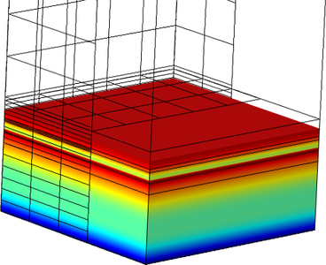
Several improvements have been implemented to speed up the discontinuous Galerkin (dG) method and to reduce its memory footprint. Speedup is primarily a result of a new mesh metric being used for the calculation of the internal time step, which is the time explicit method in dG. A second improvement in speedup has been achieved through a new mesh quality optimization procedure. This utilizes the new Avoid too small elements mesh option when generating a tetrahedral mesh in 3D (see image).
Reduction in memory is mainly achieved when running models on multicore systems. Here, a sparse assembly is used in the dG method and the required memory is almost independent of the number of CPU cores that are available. Furthermore, the memory required during initialization has been substantially reduced.
As an example, consider the Ultrasound Flow Meter with Generic Time-of-Flight Configuration tutorial model. In a test run on a desktop computer with an Intel Core™ i7 processor at 3.60 GHz with 4 cores and 32 GB of RAM, the acoustics problem is solved in 7 hours and 5 minutes and requires 6.0 GB of RAM in version 5.2a of COMSOL Multiphysics®. In version 5.3, the same study is now solved in 5 hours and 1 minute and requires 5.8 GB of RAM. This represents a speedup of roughly 30% and a slight reduction in memory. With a processor with more cores, the memory reduction running on 16 cores would then be nearly 1 GB, compared to the reduction of only 0.2 GB with 4 cores, as in this example. For reference, the model contains 7.5 million degrees of freedom (DOF).
Application Library path for examples using the improved dG method:
Acoustics_Module/Ultrasound/ultrasound_flow_meter_generic
Improved Stabilization for the Linearized Navier-Stokes Physics Interfaces
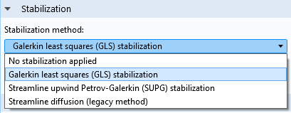
New and improved stabilization methods have been added to the Linearized Navier-Stokes interfaces. The new default stabilization scheme is the Galerkin least squares (GLS) stabilization, which highly improves the stability and convergence for solutions with coarse meshes. If desired, you can also turn off stabilization, select a Streamline upwind Petrov-Galerkin (SUPG) stabilization scheme, or select the Streamline diffusion (legacy method) scheme. The new default settings are well suited for modeling most flow-acoustic interaction problems using the Linearized Navier-Stokes interfaces. With the new stabilization scheme implemented into the Linearized Navier-Stokes interfaces, it is now possible to change the default discretization for pressure, velocity, and temperature parameters and DOF to being linear elements. This reduces the model size in many situations.
Application Library path for examples using the improved Galerkin least squares (GLS) stabilization:
Acoustics_Module/Aeroacoustics_and_Noise/helmholtz_resonator_with_flow
Reformulation of the Slip Condition
The Slip boundary condition in the Thermoviscous Acoustics and the Linearized Navier-Stokes interfaces has been reformulated to use the so-called Discontinuous Galerkin (dG) formulation, alternatively called Penalty-like formulation. The dG formulation is the new default, replacing the Lagrange multiplier-based formulation used in COMSOL Multiphysics® version 5.2a (the latter formulation can still be selected, if desired). Both formulations prevent so-called locking phenomena on curved surfaces that lead to erroneous results. The new formulation is especially well suited to solve with an iterative solver, which was not the case for the old formulation.
In cases where boundary layers are important, the default no-slip condition on the walls is the origin of the viscous boundary layer and the isothermal condition is the origin of the thermal boundary layer. It is within these acoustic boundary layers that most of the thermoviscous dissipation occurs, which is important to account for in many applications.
A slip condition imposes a no-penetration condition where no viscous boundary layer is created. Use this Slip condition in places where the viscous losses in the boundary layer are not important. This negates meshing the boundary layer and results in fewer mesh elements and DOF. Using the Slip condition is especially useful in linearized Navier-Stokes models where the interesting behavior is described by the coupling of the flow to the mean background flow, not details in the boundary layer.
Serendipity Elements in Acoustics
A variety of physics interfaces in the Acoustics Module now allow you to choose between two families of shape functions in the Discretization section: Lagrange and serendipity. The current default is to use Lagrange elements in all interfaces, except for the Solid Mechanics interface where the default is to use serendipity elements. Choosing between Lagrange and serendipity elements influences the number of DOF that are solved for, as well as the stability in models that contain distorted meshes.
When using a structured mesh, it is often beneficial to switch to serendipity shape functions, as they generate significantly fewer DOF. The accuracy is, in most cases, almost as good as when modeling with Lagrange shape functions. The Lagrange elements, however, are less sensitive to strong mesh distortions and are preferred in these cases. Using serendipity elements is only beneficial for the following element shapes, as other element shapes would result in the same number of DOF, irrespective of the choice of shape function:
- In 2D: for quadrilateral elements of discretization order higher than one
- In 3D: for hexahedral, prism, and pyramid elements of discretization order higher than one
 Example of a structured swept mesh where it can be beneficial to switch from the default Lagrange elements to serendipity elements. This makes a difference, as the swept mesh consists of prisms. In a thermoviscous acoustics simulation, using Lagrange elements results in 59,955 DOF. Switching the discretization for the velocity and the temperature to quadratic serendipity elements reduces the count to 39,955 (the pressure still uses a linear discretization in thermoviscous acoustics, which is not affected by the switch).
Preview Evaluation Plane Functionality for Far-Field and Directivity Plots
You can now use the Preview Evaluation Plane feature in far-field and directivity plots. This plots the circle (scaled) where the far-field evaluation is carried out, as well as the evaluation plane normal and reference direction vectors (the direction that represents 0 degrees in polar plots). This greatly helps to visualize and verify that the evaluation is carried out at the correct location after entering or modifying the evaluation settings.
 The preview evaluation plane and the plane's normal and reference directions for far-field plots with its corresponding settings. From the Loudspeaker Driver in a Vented Enclosure model.
Application Library path for an example that shows the preview evaluation plane:
Acoustics_Module/Electroacoustic_Transducers/vented_loudspeaker_enclosure
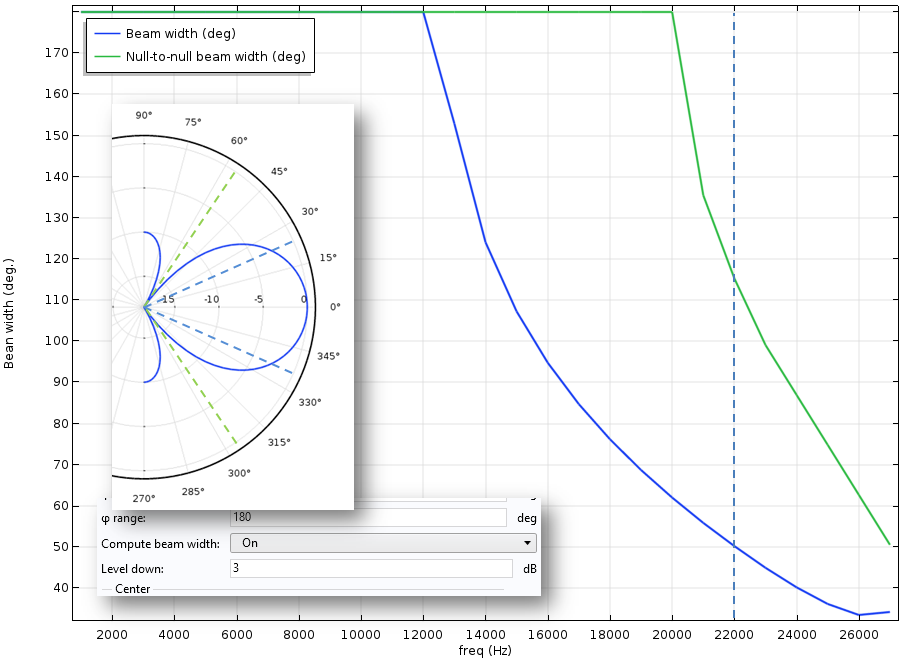
Beam Width Calculation for 1D Far-Field Plots
The beam width and the null-to-null beam width of spatial radiation patterns can now be calculated automatically. The Compute beam width functionality is available when a spatial response is plotted in a Polar Plot Group using the 1D Far-field plot.
Mode Analysis in Solid Mechanics and Coupled Acoustic-Structure Physics
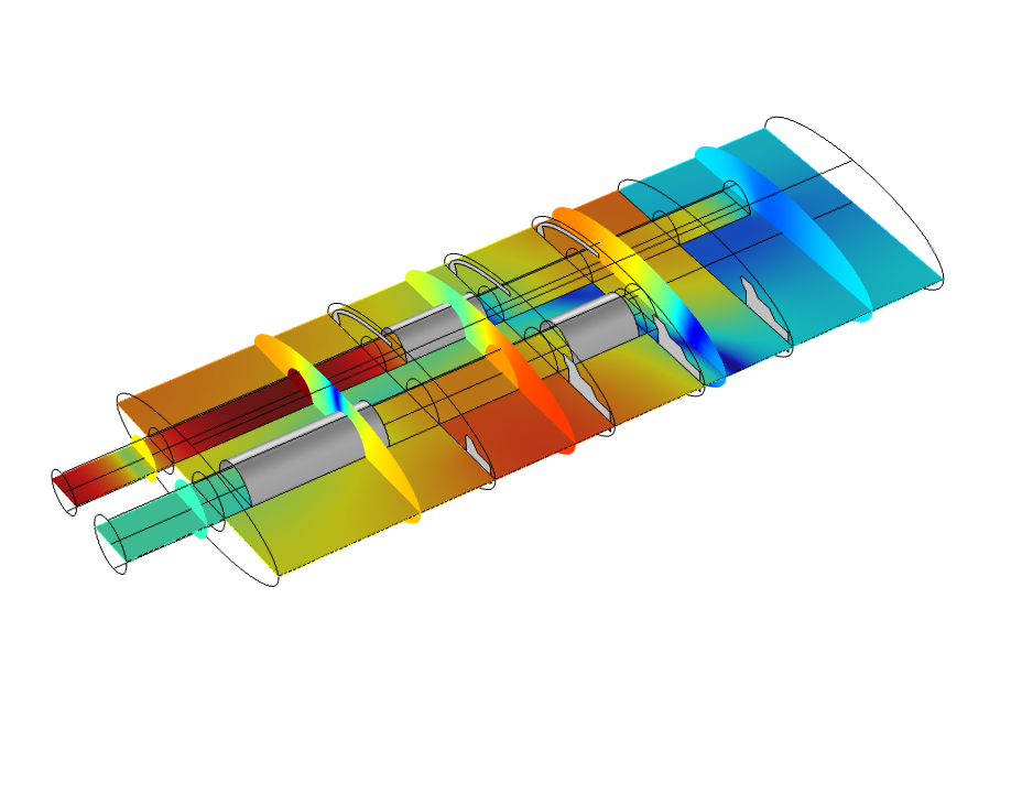
Mode analysis has been added in the Solid Mechanics interface for studying waves traveling in the out-of-plane direction for 2D structures, as well as circumferential modes in axially symmetric models. Mode analysis is particularly important in coupled acoustic-structure problems and works seamlessly in the coupled problems. This type of analysis can be used to analyze the propagating modes in applications such as waveguides, pipe systems, and mufflers.
 Coupled acoustic and structural propagating mode in a muffler chamber with thin elastic walls.
Application Library path for examples using mode analysis:
Acoustics_Module/Automotive/eigenmodes_in_muffler_elastic
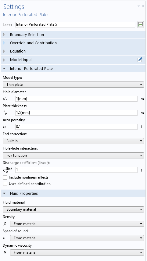
Updated Interior Perforated Plate Boundary Condition
The Interior Perforated Plate boundary condition, available in the Pressure Acoustics, Frequency Domain interface, has been updated and improved. The condition now includes full viscous and thermal loss models, hole-hole interaction using the Fok function, options to add nonlinear loss effects, and a formulation suited for both thin and thick plates. The boundary condition is typically used to model perforates in mufflers or in sound-proofing assemblies.
Sound pressure distribution in a muffler with perforates. The gray boundaries use the Interior Perforated Plate condition and the transmission loss calculated in the model is compared to measurements.
Application Library path for an examples using the Interior Perforate Plate boundary condition:
Acoustics_Module/Automotive/perforated_muffler
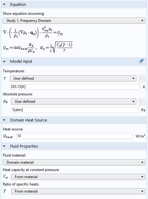
Heat Source for Pressure Acoustics
A new Heat Source condition has been added to the Pressure Acoustics interfaces. You can use this feature to represent an oscillating or pulsing heat source that will generate sound waves. The source can, for example, represent a flame in a combustion application that will generate acoustic waves in a combustion chamber or a pulsing laser beam in optoacoustic applications.
Improved Ray Acoustics in 2D Axisymmetric Geometries
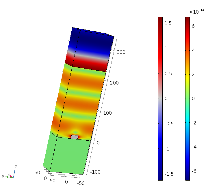
When computing ray intensity in 2D axisymmetric models, the wavefront associated with the propagating ray is now treated as a spherical or ellipsoidal wave, instead of a cylindrical wave, which was only ever an appropriate simplification in true 2D models. In other words, the principal radius of curvature associated with the azimuthal direction is computed for all rays. This improvement leads to more realistic calculations of the ray intensity in 2D axisymmetric models. Typical applications are in underwater acoustic simulations, as illustrated in the associated figure.
Additionally, dedicated features have been included to release rays from edges, points, or at specified coordinates along the axis of symmetry. When using one of these dedicated release features, a built-in option is available to release rays in an anisotropic hemisphere such that each ray approximately subtends the same solid angle in 3D.
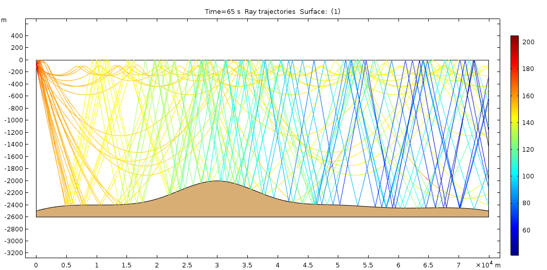 An underwater ray tracing model in a 2D axisymmetric geometry with graded media (speed of sound is depth dependent) and domain attenuation. Axisymmetric models are often used as approximations to full 3D applications in underwater acoustics.
Application Gallery link for an example using the ray acoustics in 2D axisymmetries:
Underwater Ray Tracing Tutorial in a 2D Axisymmetric Geometry
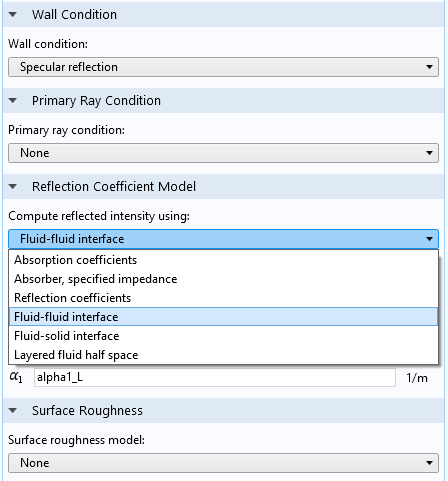
New Reflection Coefficient Models for Acoustics Ray Tracing
The Wall feature now has several built-in models to calculate the reflection coefficient at specular reflections including a Fluid-fluid interface, Fluid-solid interface, and Layered fluid half space models. These new models are ideal for setting up boundary conditions in underwater ray tracing applications. They complement the Absorber, specified impedance model, typically used in room acoustics to model absorbing panels. The attenuation in the propagation fluid and the attenuation in the domains, modeled by the boundary conditions, are also included to calculate a correct phase shift at the reflections. All boundary conditions can be extended with a Surface Roughness option using the Rayleigh roughness model.
Ray Termination Feature
The new Ray Termination feature can be used to annihilate rays without requiring them to stop at a boundary. Rays can be terminated if their intensity or power becomes smaller than a specified threshold or if they stray too far from the model geometry. You can use this feature to avoid using excessive computational resources on rays that have become attenuated due to the presence of absorbing media, rays that have extremely low intensity due to interaction with curved or absorbing surfaces, or stray rays that have escaped from the geometry.
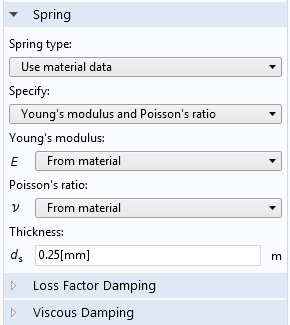
Elastic Layers Described by Material Data
You can now prescribe the elastic properties of a spring foundation or a thin elastic layer with material data such as Young's modulus and Poisson's ratio together with a given thickness of the layer. This simplifies, for example, the modeling of adhesive layers with known material properties. When using the material data and thickness as input, the strains in the elastic layer are also available as results.
New Framework for Inelastic Strains in Geometrically Nonlinear Analyses
A new framework and more rigorous handling of decomposition into elastic and inelastic deformations has been implemented for cases of geometric nonlinearity. Previous versions of the COMSOL® software used an additive decomposition approach, with a few exceptions such as for large-strain plasticity analyses, which use a multiplicative decomposition approach.
Multiplicative decomposition is now also available for:
- Thermal Expansion
- Hygroscopic Swelling
- Initial Strain
- External Strain
- Viscoplasticity
- Creep
Multiplicative decomposition of deformation gradients is now the default option for all inelastic contributions in studies where geometric nonlinearity is active. The main advantage is that it is possible to handle several large inelastic strain contributions in a material. Furthermore, linearization will be more consistent as, for example, it is now possible to accurately predict the shift in eigenfrequencies caused by pure thermal expansion. If you want to switch to the behavior of previous versions of the COMSOL Multiphysics® software, the new Additive strain decomposition check box can be selected in the Settings window for the respective material models.
As part of this improvement, the External Strain attribute under the Linear Elastic Material and Nonlinear Elastic Material nodes has been expanded with several new options. These options allow for supplying inelastic strains in several forms and you can also transfer inelastic strains from other physics interfaces to this attribute. Additionally, an External Strain attribute with similar properties has been added to the Hyperelastic Material.
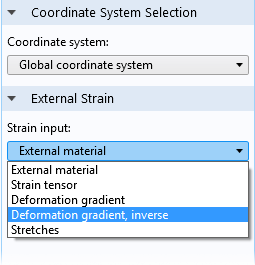
Enhancements and Important Bug Fixes
- Several of the pressure acoustics boundary conditions are now sorted in new submenus for better overview
- Far-field SPL calculation speedup for Directivity and Far-field plots
- The Background acoustic fields feature is now also available in the transient version of the Linearized Euler and Linearized Navier-Stokes interfaces
- Interior Normal Displacement and Interior Normal Velocity boundary conditions have been added to the Pressure Acoustics interfaces to complete the interior boundary conditions list
- Updated conditions in the Thermoviscous Acoustics, Linearized Navier-Stokes, and Linearized Euler interfaces at the symmetry axis in 2D axisymmetric models has been included
- An update of the formulation in the Thermoviscous Acoustics interfaces has been enacted to be valid for media with space-dependent material properties
- The Aeroacoustic-Structure Boundary multiphysics coupling now couples the Linearized Navier-Stokes interface to structures (solids, shells, and membranes) in the time domain
New Tutorial: Helmholtz Resonator with Flow, Interaction of Flow and Acoustics
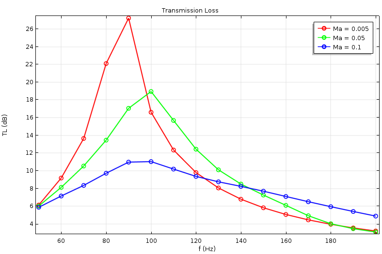
Helmholtz resonators are used in exhaust systems, as they can attenuate a specific narrow frequency band. The presence of a flow in the system alters the acoustic properties of the resonator and the transmission loss of the subsystem. In this tutorial model, a Helmholtz resonator is located as a side branch to a main duct. The transmission loss through the main duct is investigated when a flow is introduced.
The mean flow is calculated with the SST turbulence model for Ma = 0.05 and Ma = 0.1. The acoustics problem is then solved using the Linearized Navier-Stokes, Frequency Domain (LNS) interface. The mean flow velocity, pressure, and turbulent viscosity are coupled to the LNS model. Results are compared to measurements found in a journal paper and the amplitudes and resonance locations show good agreement with the measurement data (as seen in the 1D plot). The balance between attenuation and flow effects needs to be modeled rigorously in order for the resonance location to be correct.
Note: This model requires both the Acoustics Module and the CFD Module.
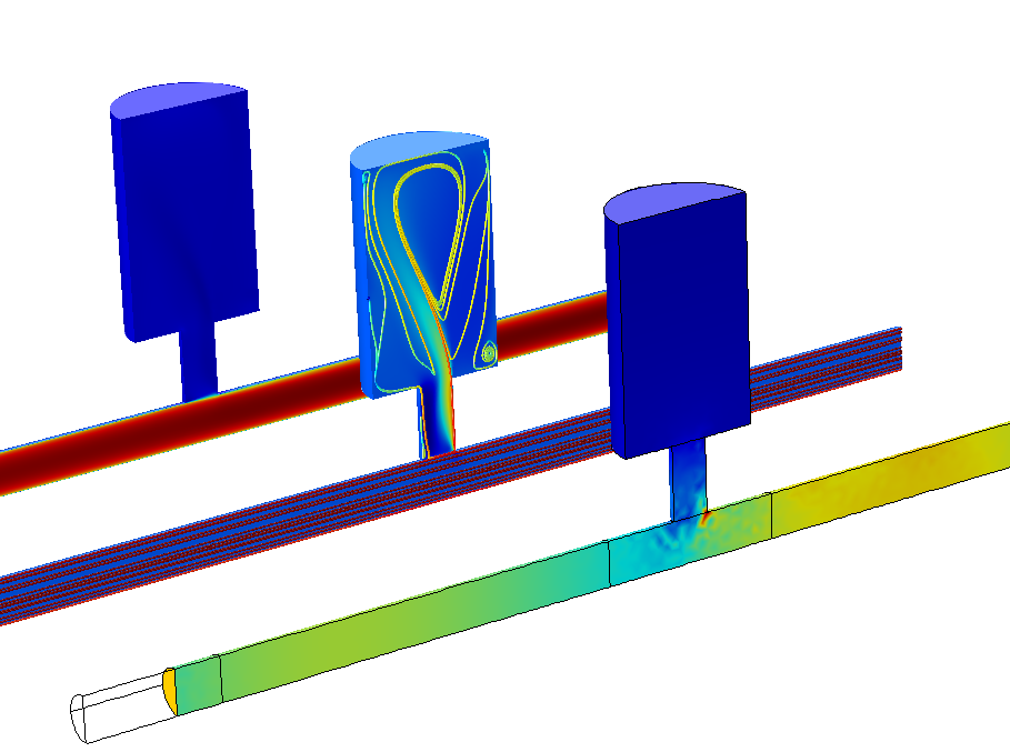 Acoustic sound pressure level distribution (front), surface streamlines (middle), and the background flow velocity amplitude (back) in a Helmholtz resonator located as a side branch to a main duct.
Application Library path:
Acoustics_Module/Aeroacoustics_and_Noise/helmholtz_resonator_with_flow
New Tutorial: Ultrasonic Flow Meter with Piezoelectric Transducers, Coupling Between FEM and DG
Ultrasonic flow meters are used to determine the velocity of a fluid flowing through a pipe by sending an ultrasonic signal across the flow at a skew angle. In the case of no flow, the transmitting time between the transmitter and the receiver is the same for the signals sent in the upstream and the downstream directions. Otherwise, the downstream-traveling wave moves faster than the upstream-traveling wave, which can be used to ascertain the flow. In many cases, piezoelectric transducers are used to send and receive the ultrasonic wave.
This tutorial model shows how to simulate an ultrasonic flow meter with piezoelectric transducers in the simplified no-flow case. The finite element method (FEM) is used to model the piezoelectric transducers, whereas the modeling of the ultrasonic wave propagation is based on the discontinuous Galerkin (dG) method. The whole model is split into two submodels. An FEM to dG one-way coupling is used to send the wave from the transmitter, and a dG to FEM one-way coupling is used to simulate the receiver.
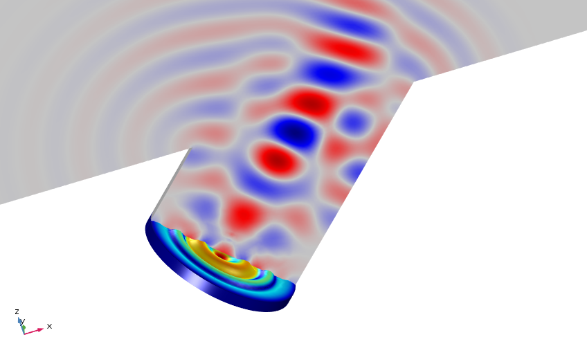 Acoustic signal generated in a flow meter by a piezoelectric transducer with a matching layer.
Application Library path:
Acoustics_Module/Ultrasound/flow_meter_piezoelectric_transducers
New Tutorial: Gaussian Pulse Absorption by Perfectly Matched Layers; Pressure Acoustics, Transient
This tutorial simulates a standard test and benchmark model for perfectly matched layers (PMLs) as absorbing boundary conditions in the time domain. It involves the propagation of a transient Gaussian pulse with no flow. The Pressure Acoustics, Transient interface is used together with PMLs to reduce the computational domain and suppress the reflections from the artificial boundaries. An acoustic pulse is generated by an initial Gaussian distribution at the center of the computational domain. The analytical solution to the problem is used to validate the solution, showing very good agreement.
Application Library path:
Acoustics_Module/Tutorials/gaussian_pulse_perfectly_matched_layers
New Tutorial: Noise Radiation by a Compound Gear Train
Predicting the noise radiation from a dynamic system gives designers an insight into the behavior of moving mechanisms early in the design process. For example, consider a gearbox in which the change in the gear mesh stiffness causes vibrations. These vibrations are transmitted to the gearbox housing through shafts and joints. The vibrating housing further transmits energy to the surrounding fluid, resulting in acoustic wave radiation.
This tutorial model simulates the noise radiation from the housing of a gear train. First, a multibody dynamics analysis is performed in the time domain to compute the housing vibrations at the specified driver shaft speed. Then, an acoustics analysis is performed at a selected frequency to compute the sound pressure levels in the near, far, and exterior fields using the housing's normal acceleration as a noise source.
Note: This model also requires the Multibody Dynamics Module and the Structural Mechanics Module.
Application Library path:
Acoustics_Module/Vibrations_and_FSI/gear_train_noise
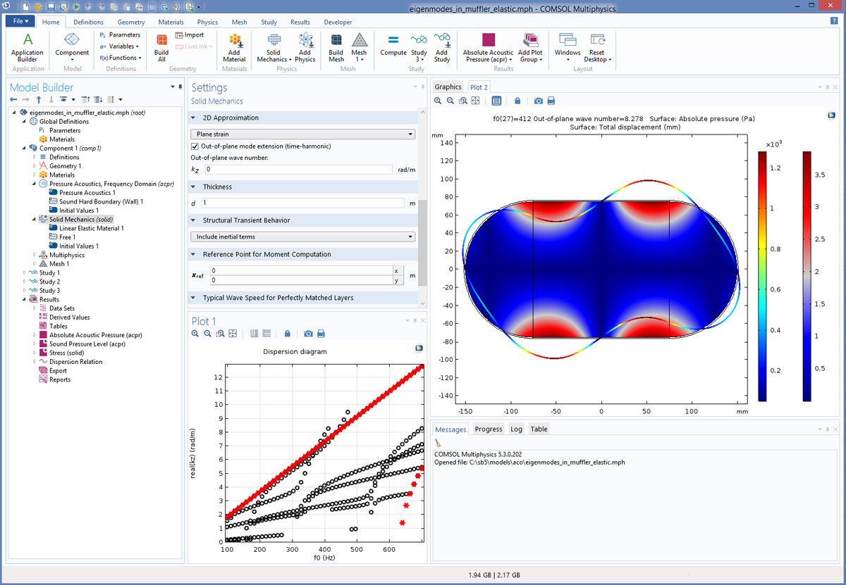
New Tutorial: Eigenmodes in a Muffler with Elastic Walls
This tutorial model, an extension of the Eigenmodes in a Muffler model, solves a 2D analysis of propagation modes in the chamber of a muffler with thin elastic walls. This acoustic-structure multiphysics tutorial uses the new Mode Analysis feature to study the waves traveling in the out-of-plane direction. The results include the absolute pressure and sound pressure level in the muffler, the displacement and stress in the elastic walls, and a 1D dispersion relation plot.
 The absolute pressure (Wave plot) and deformation (Rainbow plot) shown in a muffler with elastic walls.
Application Library path:
Acoustics_Module/Automotive/eigenmodes_in_muffler_elastic
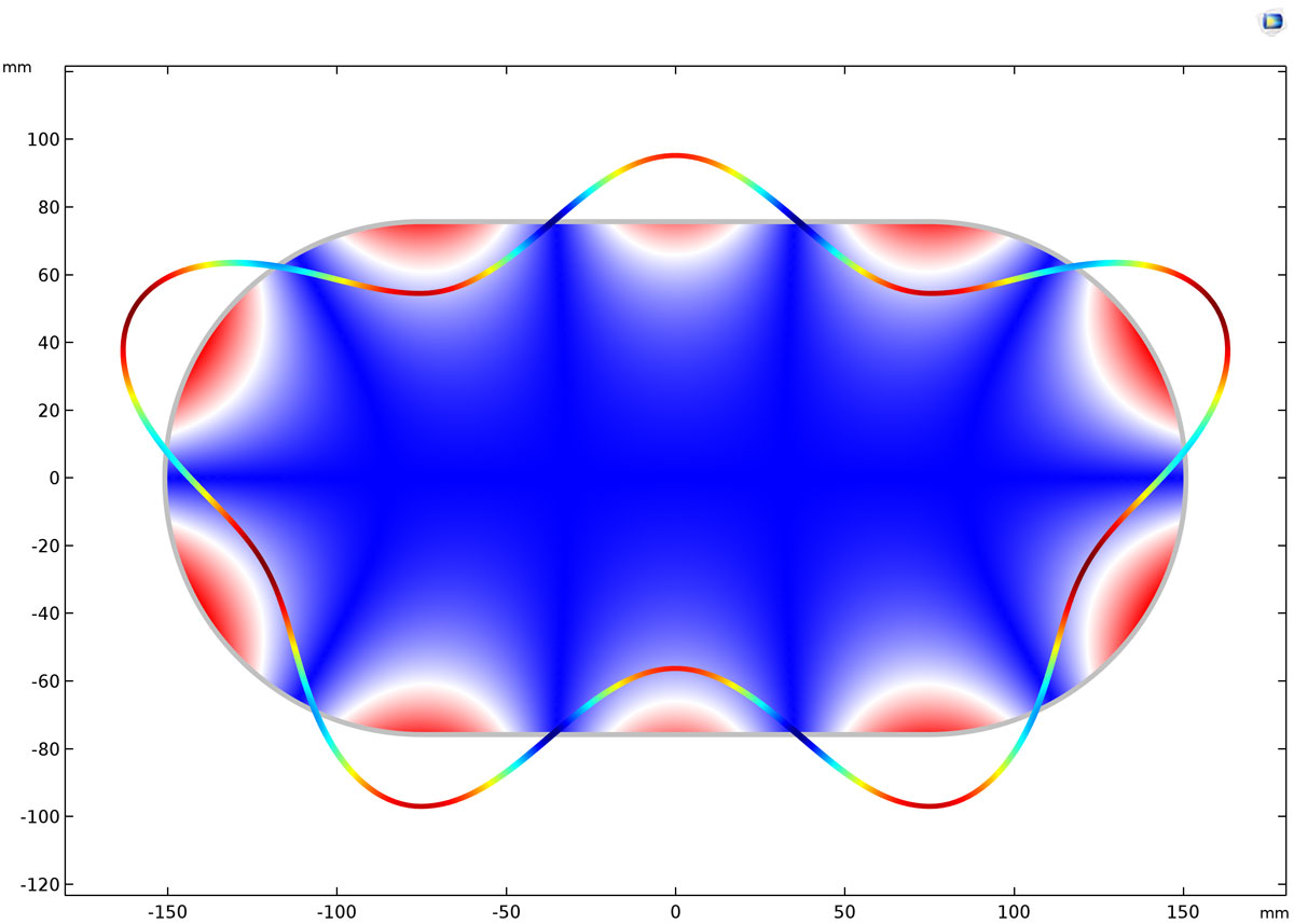
New Tutorial: Magnetic Circuit Topology Optimization
This tutorial model presents an example of topology optimization of the magnetic circuit of a loudspeaker driver. Using topology optimization, you can find the shape of a nonlinear iron yoke in order to maximize its performance and, at the same time, minimize the weight such that it is smaller than the original design.
Note: This model requires the AC/DC Module and the Optimization Module.
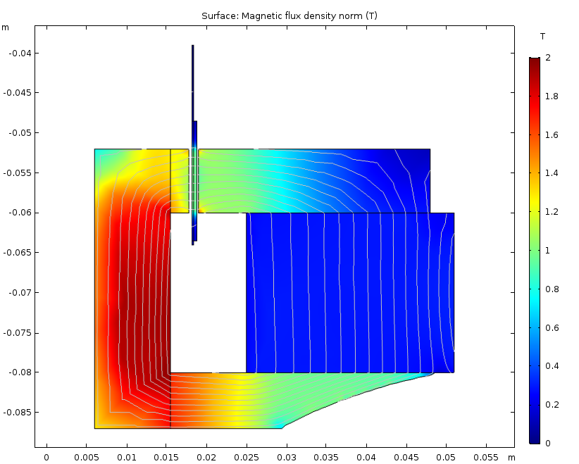 Magnetic flux density plotted in the optimized magnetic circuit geometry with 2D axisymmetry. The geometry is very similar to the motor in the loudspeaker driver tutorial model found in the Acoustics Module.
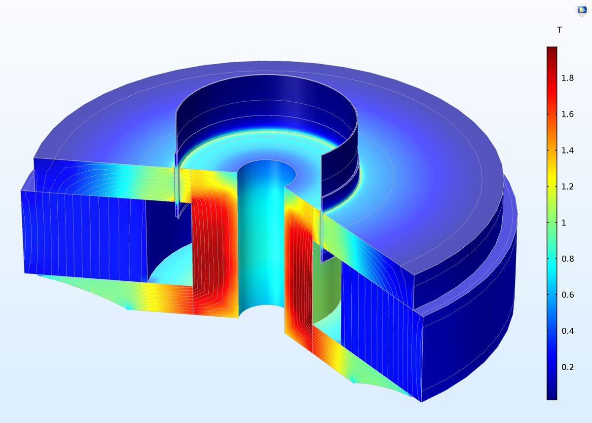 The magnetic flux density plotted in the optimized magnetic circuit geometry, solved with 2D axisymmetry and revolved 225 degrees into 3D space.
Application Library path:
AC/DC_Module/Other_Industrial_Applications/magnetic_circuit_topology_optimization
New Tutorial: Nonlinear Slit Resonator, Coupling Acoustics and CFD
In many applications, acoustic waves interact with surfaces that have small perforations or slits. This can be in muffler systems, sound-proofing structures, liners for noise suppression in jet engines, or grilles and meshes. At medium-to-high sound pressure levels, the local particle velocity in the narrow region of the perforate or slit can be so large that the linear assumptions of acoustics break down. Typically, vortex shedding takes place in the vicinity of that region, which leads to nonlinear losses, and in audio applications, it leads to nonlinear distortion of sound signals. The nonlinear effects are sometimes included through semiempirical parameters in analytical transfer impedance models for perforates.
In this tutorial, a narrow slit is located in front of a resonator volume and the losses are modeled directly. The model couples pressure acoustics and the Laminar Flow interface in a transient simulation in order to model the complex nonlinear losses associated with the vortex shedding. The incident acoustic field has an amplitude corresponding to 155 dB SPL.
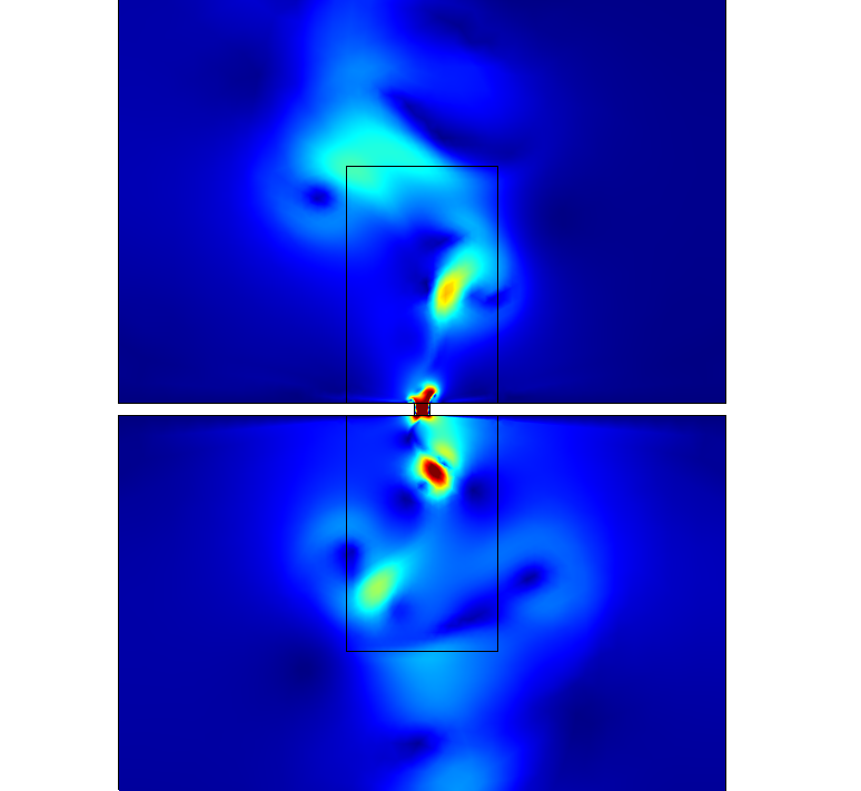 Vortex shedding at the narrow slit induced by the incident high-amplitude acoustic waves.
Application Gallery link:
Nonlinear Slit Resonator: Coupling Acoustics and CFD
New Tutorial: Multilayered Porous Material, Poroelastic Waves with Thermal and Viscous Losses (Biot-Allard Model)
In applications where pressure and elastic waves propagate in porous materials filled with air, both thermal and viscous losses are important. This is typically the case in insulation materials for rooms, lining materials in car cabins, or foams used in headsets and speakers. Another example is porous materials in mufflers in the automotive industry.
In many cases, these materials can be modeled using the Poroacoustic models (equivalent fluid models, only solving for the pressure) implemented in the Pressure Acoustics interface. In a simplified model in the Acoustics Module, the Poroelastic Waves interface is based on the classic Biot theory used in Earth sciences. This assumes that the saturating fluid is a liquid (water) and the model only includes viscous losses. The material inputs are also different from those typically supplied with acoustic insulation materials.
Yet, a Poroacoustic model does not capture all of the effects and sometimes it is necessary to also include elastic waves in the porous matrix. This is covered by the Biot-Allard theory for modeling poroelastic waves. The model based on this theorem can be selected in the Poroelastic Waves interface.
 Deformation of the porous matrix inside a multilayered porous structure.
Application Gallery link:
Multilayered Porous Material: Poroelastic Waves with Thermal and Viscous Losses (Biot-Allard Model)
New Tutorial: Acoustics of a Pipe System with 3D Bend and Junction
A new tutorial shows how to model the propagation of acoustic waves in large pipe systems by coupling Pipe Acoustics to Pressure Acoustics. The tutorial is set up in both the time domain and the frequency domain. 1D pipe acoustics is used to model the propagation in the long straight pipe portions. A 3D model of a pipe junction and pipe bend is coupled to the 1D pipe model in order to model these parts in detail. This kind of model can be used to model and predict the response of pipe systems such as when detecting leaks or deformations, for example, and is relevant in the oil and gas industry or in water delivery pipe systems.
Application Gallery link:
Acoustics of a Pipe System with 3D Bend and Junction
New Tutorial: Topology Optimization of Acoustic Modes in a 2D Room
This tutorial model introduces the use of topology optimization in acoustics. The goal of the optimization is to find the material distribution (solid or air) in a given design domain that minimizes the average sound pressure level in an objective region of a 2D room. The optimization is carried out for a single frequency.
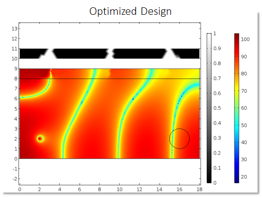 Optimized material distribution (gray scale) and sound pressure level distribution after optimization (color scale).
Application Gallery link:
Topology Optimization of Acoustic Modes in a 2D Room
New Tutorial: Anechoic Coating
Anechoic coatings are used to reduce visibility to sonar detection, useful for submarines as an example. This tutorial model calculates the reflection, absorption, and transmission properties of an anechoic coating on a steel plate. The considered setup was presented in V. Leroy, A. Strybulevych, M. Lanoy, F. Lemoult, A. Tourin, and J. H. Page, "Superabsorption of acoustic waves with bubble metascreens," Physical Review B, vol. 91, no. 2, 2015.
 Local deformations in the coating and the steel plate.
Application Gallery link:
Anechoic Coating
New Tutorial: Acoustics of Coupled Rooms Using the Acoustic Diffusion Equation
This verification model analyzes the acoustics of two coupled rooms using the Acoustic Diffusion Equation interface of the Acoustics Module. The results of the model agree with analytical results that are validated against measurements in a reference paper.
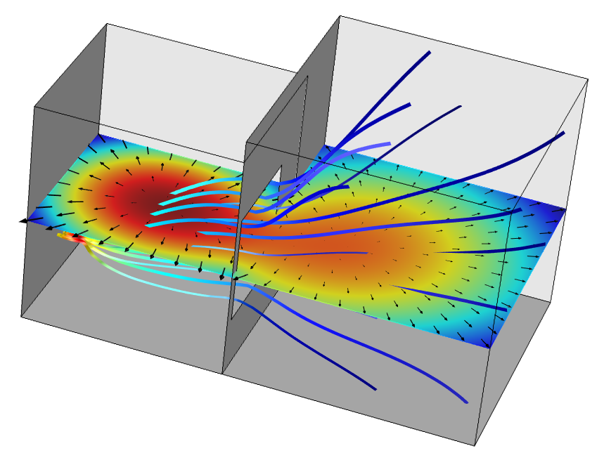 Energy density and local energy flow in two acoustically coupled rooms.
Application Gallery link:
Acoustics of Coupled Rooms using the Acoustic Diffusion Equation
Intel and Intel Core are trademarks of Intel Corporation or its subsidiaries in the U.S. and/or other countries.