

When we study and prototype a phased array antenna for high-speed and high-data-rate communication, we can save time and computational costs by using an antenna array factor. This way, we don’t need to analyze the entire structure through a full 3D wave equation.
Antenna Applications in IoT, IoS, SatCom, and 5G
There is a common theme among today’s trendy RF buzzwords, such as internet of things (IoT), internet of space (IoS), satellite communication (SatCom), and 5G: The need for wireless communication that can provide a higher data rate with an operating frequency and bandwidth much higher and wider, respectively, than what it used to be.
When we send or receive informative signals carried over a 5G mobile network, where its expected operating frequency is much higher than that of a traditional mobile system, we inevitably suffer from significant electromagnetic wave attenuation, causing signal integrity issues. In order to make the electromagnetic wave travel a longer distance with the limited amount of power in a communication system, it is necessary to deploy a high-gain antenna that shapes the far-field radiation pattern like a very sharp, pencil-like beam. This enables us to reach longer distances for delivering uninterrupted information.
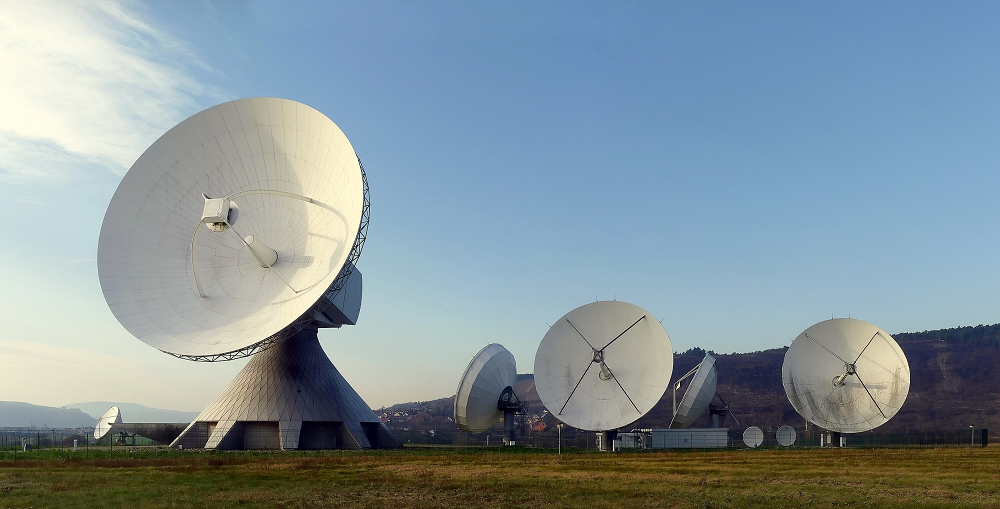
Large dish antennas allow us to communicate over a long distance. Image in the public domain, via Wikimedia Commons.
Aperture antennas, such as dish and horn antennas, would provide a high-enough gain for these purposes. The very sharp far-field radiation pattern from high-gain antennas has a very narrow angular scanning range, and the visible area of an electromagnetic wave is limited. To enhance the area covered for communication, its scanning capability can be extended by rotating the antenna mechanically with a gimbal. However, aperture antennas require a substantial amount of space, volume-wise, to install, and may not be suitable for use in consumer electronics — You do not want to add a big dish antenna to your cellphone!
A monopole antenna array showing beam scanning capability.
An antenna array is, simply put, a bunch of antennas connected by a specific space and phase configuration. Arrays can overcome the obstacles mentioned above, and they can be conformal and miniaturized based on the antenna element type, forming an array and material properties.
It is important to choose a proper antenna element if miniaturization is a design factor. The design specification may decide what type of antenna element to deploy.
The Benefit of Using an Array Factor
Though the volume of an antenna array is smaller than that of an aperture-type antenna, its computational cost for simulation is still high compared to a single antenna study. Without running a full 3D model simulation over the entire structure and sacrificing the accuracy of the analysis too much, the far-field radiation pattern of the antenna array can still be estimated from the radiation pattern of a single antenna element by multiplying the array factor.
The uniform array factor expression in a 3D model is defined as
where nx, ny, and nz are the number of array elements along the x-, y-, and z-axis, respectively. The terms dx, dy, and dz are the distance between array elements in terms of the wavelength used in a simulation. The terms alphax, alphay, and alphaz are the phase progression in radians.
In the above array factor expression, the input power is not normalized. If an antenna array is excited with a single input power distributed by a feed network, it needs to be scaled accordingly.
One of the advantages of using the COMSOL Multiphysics® software is that you can type any kind of equation for the postprocessing expression. When the expression is complicated, it can be addressed using a simulation application or model methods.
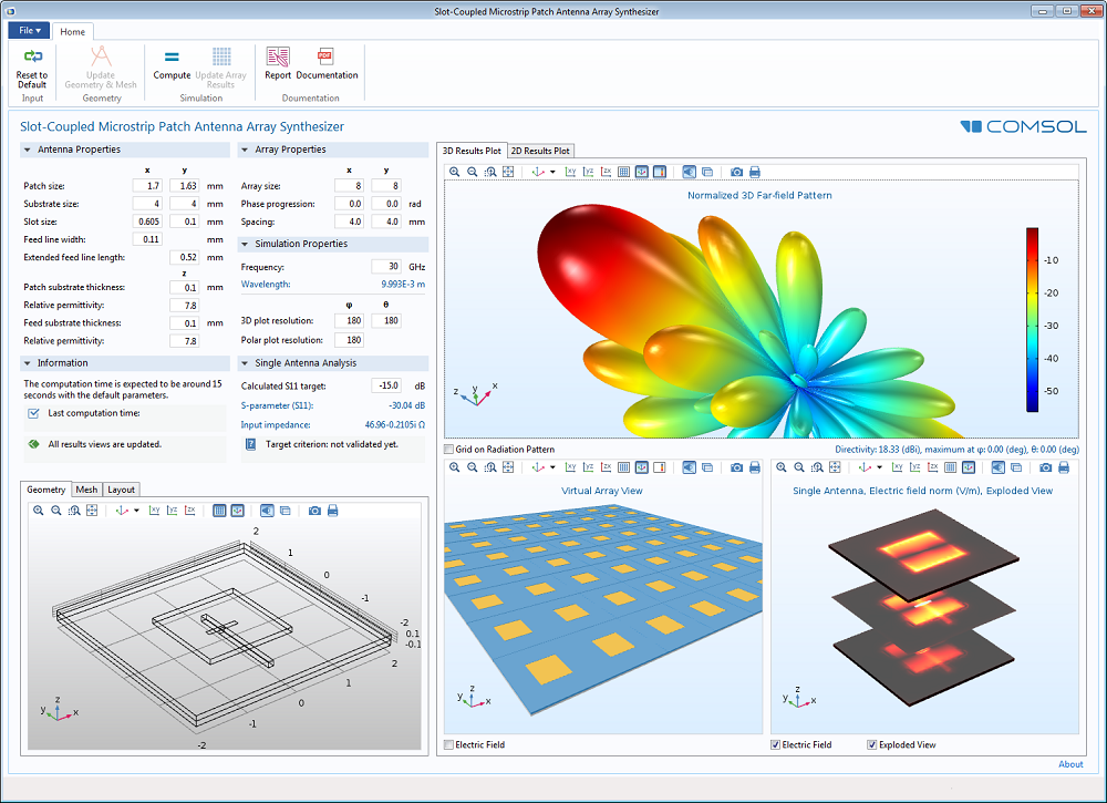
The user interface of an antenna array simulation application with an 8×8 virtual array, electric field distribution, and 3D far-field radiation pattern view.
By multiplying the array factor equation to the antenna far-field gain variable, emw.gaindBEfar, you can compute the far-field gain of the antenna array.
Array Factor Function in the RF Module
Typing a long expression of an equation or programming even a simple code using method functionality could be a hindrance for a quick study. Fortunately, the RF Module, an add-on to COMSOL Multiphysics, offers an array factor postprocessing function. After a single antenna simulation with a far-field domain/calculation physics feature, the 3D uniform array factor function is accessible under Definitions > Functions from the postprocessing context menu for the plot expression as
af3(nx, ny, nz, dx, dy, dz, alphax, alphay, alphaz)
The definition of the input arguments is the same as in the above uniform array factor equation, and the following table explains the impact on the resulting plot.
| Effect | Input Argument | Number of array elements | Antenna gain |
|---|---|
| Distance between array elements | Antenna gain; sidelobe level |
| Phase progression | Main lobe steering direction |
The effect of input parameters on the radiation pattern.
The evaluation of a virtual 8×8 antenna array that has a main beam in the z-axis is expressed as
emw.gaindBEfar + 20*log10(emw.af3(8, 8, 1, 0.48, 0.48, 0, 0, 0, 0)) + 10*log10(1/64)
It is calculated in the dB scale, and the multiplication between the array factor and the single antenna gain is done by summation in the expression.
| Input Argument | Description | Value | Unit |
|---|---|---|---|
nx
|
Number of elements along the x-axis | 8.00 | Dimensionless |
ny
|
Number of elements along the y-axis | 8.00 | Dimensionless |
nz
|
Number of elements along the z-axis | 1.00 | Dimensionless |
dz
|
Distance between array elements along the x-axis | 0.48 | Wavelength |
dy
|
Distance between array elements along the y-axis | 0.48 | Wavelength |
dz
|
Distance between array elements along the z-axis | 0 | Wavelength |
alphax
|
Phase progression along the x-axis | 0 | Radian |
alphay
|
Phase progression along the y-axis | 0 | Radian |
alphaz
|
Phase progression along the z-axis | 0 | Radian |
Array factor input arguments of a virtual 8×8 array antenna for the main beam along the z-axis.
The above expression is made under the assumption that the antenna array is fed by a uniform distribution network with a single input power source. It is necessary to scale it by a factor of 10*log10(1/total number of elements).
When nonzero phase progression values are used, the direction of the main beam, the maximum radiation, can be pointed toward a desirable direction. The distance between the array elements is 0.48 wavelengths. When the distance is between 0.45 and 0.5 wavelengths, it is expected to have a sidelobe level of approximately -12 to -15 dB.
The following equation helps define the phase progression value as a function of the angle from the major axis, so you can easily point the scanning direction.
where k is wavenumber, d is the distance between antenna elements, and theta is the angle from the axis.
To generate the beam with the maximum direction at 60 degrees from the x-axis, alphax (in the array factor function) is set to
-2*pi*0.48*cos(pi/3)
The Microstrip Patch Antenna tutorial in the Application Gallery shows how the single antenna radiation pattern can be evolved using the array factor.
The following polar plot compares three radiation patterns:
- The gain of a single microstrip patch antenna
- The pattern of a uniform array factor set to have the main lobe direction 60 degrees from the x-axis and 30 degrees from the z-axis
- The synthesized gain of an 8×8 microstrip patch antenna array
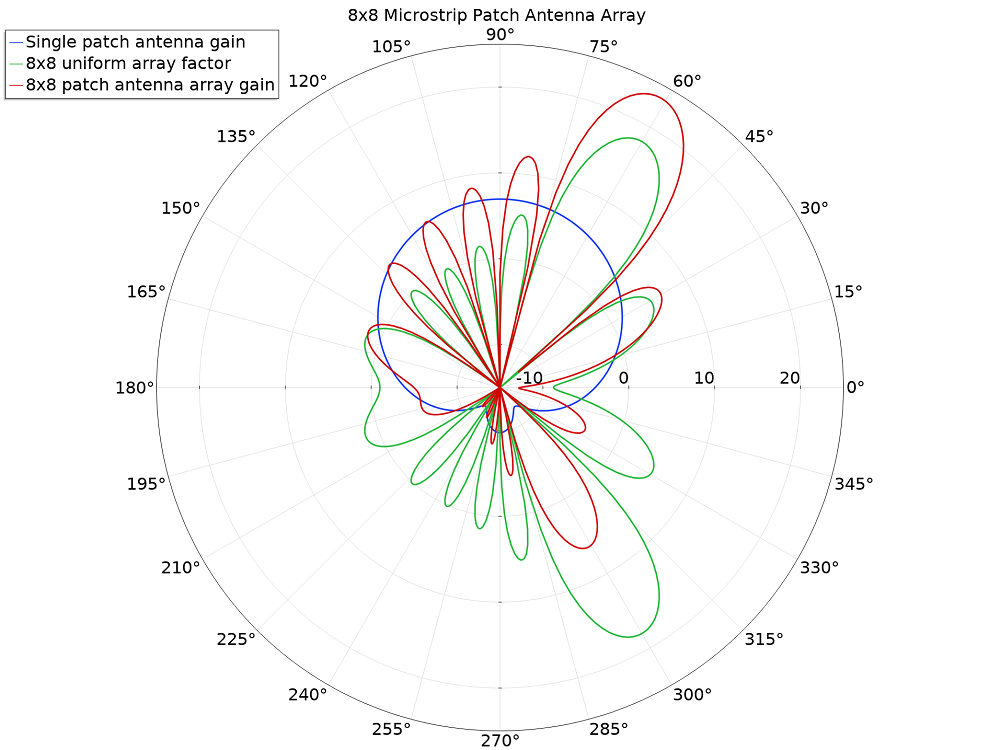
The single patch antenna gain, 8×8 uniform array factor, and 8×8 microstrip patch antenna array gain plotted in dB scale.
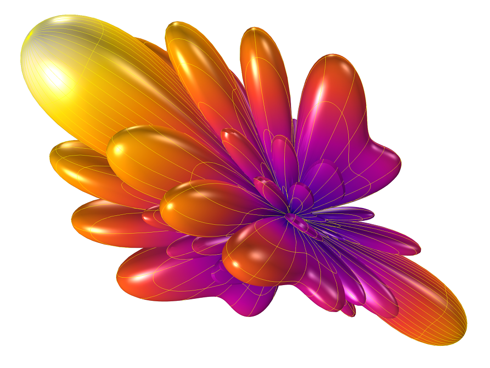
The far-field gain pattern of a virtual 8×8 microstrip patch antenna array. The minimum range for the plot may change the visual sharpness of the main beam pattern.
The Beauty of Postprocessing an Antenna Array Simulation
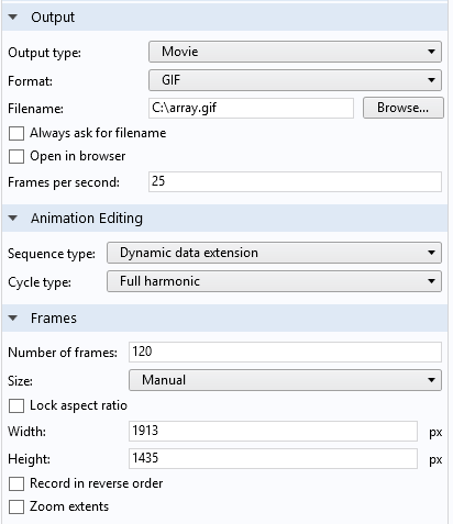
The various postprocessing options in COMSOL Multiphysics enable you to efficiently study your antenna prototype. Using the Full harmonic dynamic data extension for the animation sequence type in the animation settings is one very useful way to examine the beam steering feasibility without running the simulation at every angular scanning point.
 l
l
Animation Settings window. Dynamic data extension is used to sweep the internal phase variable.
For time-harmonic, frequency-domain simulations, the solution of dependent variables can be evaluated at an arbitrary angle (phase). The full harmonic dynamic data extension changes the internally defined “root.phase” variable from 0 to 2 pi while producing the animation.
The following expression generates the animation of the 8×8 microstrip patch antenna array, scanning the 180-degree range from the z-axis to the positive x-axis via the negative x-axis.
emw.gaindBEfar + 20*log10(emw.af3(8, 8, 1, 0.48, 0.48, 0, -2*pi*0.48*cos(phase+pi/2), 0, 0)) + 10*log10(1/64)
The far-field gain pattern of the 8×8 microstrip patch antenna array. The main beam is moving along an axis.
The scanning trajectory does not have to follow a line or a rectangular grid. The rotating main beam pattern around the z-axis of a 12×12 microstrip patch antenna array can be produced using the next expression:
emw.gaindBEfar + 20*log10(emw.af3(12, 12, 1, 0.48, 0.48, 0, -2*pi*0.48*cos(pi/2-pi/8*cos(phase)), -2*pi*0.48*cos(pi/2-pi/8*sin(phase), 0)) + 10*log10(1/144)
The far-field gain pattern of a 12×12 microstrip patch antenna array. The main beam is moving along a circular orbit.
The main beam is tilted pi/8 radian from the axis and rotating around the axis in the animation.
Concluding Remarks
The 3D full-wave simulation for a large antenna array system is memory intensive, increasing the computation time and cost. By using an asymptotic approach as discussed, by multiplying the far-field postprocessing variable of a single antenna element with a uniform array factor, you can quickly estimate the radiation pattern analysis of the antenna array. However, this approach does not address the field coupling among the array elements. Therefore, it is only applicable for fast prototype feasibility studies. The full-wave analysis over the entire array structure may be required to examine the gain and sidelobe level precisely.
Additional Resources
Check out these tutorial models to study antenna arrays via simulation:


Comments (2)
Robert Malkin
April 4, 2019Will something similar be available for acoustics in the future?
Mads Herring Jensen
April 30, 2019Hi Robert, this is the first time we receive this request. Could you tell me what the application in acoustics would be? I think that you can most probably set something similar up with the existing tools and a few user-defined expressions.