
A memory-efficient physics interface for modeling the propagation of elastic waves in solids (vibrations in structures) is available in the COMSOL Multiphysics® software as of version 5.5. The Elastic Waves, Time Explicit interface is based on a higher-order discontinuous Galerkin method with a time-explicit time integration scheme. This enables efficient multicore computation of acoustically large models. The interface is multiphysics enabled and couples to fluid domains. Today, we will explore how to use this interface, discuss best practices, and showcase some tutorials.
About the Elastic Waves, Time Explicit Interface
The Elastic Waves, Time Explicit interface is dedicated to transient linear elastic wave propagation problems over large domains containing many wavelengths. It is suited for time-dependent simulations with arbitrary time-dependent sources and fields. The interface is based on the discontinuous Galerkin method (dG-FEM) and uses a time-explicit solver.
In general, the Elastic Waves, Time Explicit interface is suited for modeling the propagation of elastic waves over large distances relative to the wavelength, such as ultrasound propagation like nondestructive testing (NDT) applications or seismic wave propagation in soil and rock.
The interface exists in 2D (generalized plane strain) and 3D, and includes absorbing layers that are used to set up effective nonreflecting boundary conditions (sponge layers; see below). The user interface and boundary conditions mirror the features available in the Solid Mechanics interface when applicable to wave propagation problems. The interface supports damping, as well as isotropic, orthotropic, and anisotropic solid material formulations.

User interface for the Elastic Waves, Time Explicit interface, here shown with the Ground Motion After Seismic Event tutorial model.
When adding the Elastic Wave, Time Explicit physics interface, it is found under the Acoustics > Elastic Waves branch (see the image below). Note that this is a new category that was added in COMSOL® version 5.5 to accommodate the new physics interface.
This category also includes two of the existing finite element (FEM) based interfaces. The Poroelastic Waves interface is focused on the propagation of coupled acoustic and structural waves in porous materials. There is also a shortcut to add the Solid Mechanics interface, as it is also used for modeling elastic waves, which is why “elastic waves” has been added to the name when accessing it via the Acoustics branch.
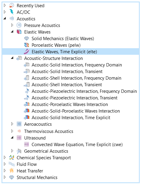
Location of the new interface in the Acoustics > Elastic Waves folder in the Add Physics wizard.
The Governing Equations
The model solves the governing equations for a general linear elastic material in a velocity-strain formulation
& \rho \frac{\partial \mathbf{v}}{\partial t} – \nabla\cdot\mathbf{S} = \mathbf{F}_\textrm{v} \\
& \frac{\partial \mathbf{E}}{\partial t} – \frac{1}{2}[\nabla \mathbf{v} – (\nabla \mathbf{v})^\textrm{T}] = \mathbf{0} \\
& \mathbf{S} = \mathbf{C}:\mathbf{E}
\end{align}
where \mathbf{v} is the velocity, \rho the density, \mathbf{S} the stress tensor, \mathbf{E} the strain tensor, \mathbf{C} is the elasticity tensor (or stiffness tensor), and \mathbf{F}_\textrm{v} is a possible body force.
The equations are valid for both isotropic and anisotropic material data. Dissipation can be added to the model in the form of Rayleigh damping. This adds additional right-hand side terms to the equation of motion (first equation) with a mass and stiffness damping term.
Multiphysics Capabilities
The new interface is multiphysics enabled and can be coupled to the Pressure Acoustics, Time Explicit physics interface for modeling large vibroacoustic or acoustic-structure interaction (ASI) problems in the time domain.
For setting up the coupling, a new Acoustic-Structure Interaction, Time Explicit multiphysics feature is available. To take full advantage of the time-explicit formulation, the use of so-called nonconforming meshes (meshes that are discontinuous at a boundary) is essential when coupling domains with different properties (this is discussed further below). This is achieved through the new Pair Acoustic-Structure Boundary, Time Explicit multiphysics coupling that handles geometric assemblies (see image below). The use of nonconforming meshes is a natural extension and use of the properties of the discontinuous elements.

User interface for the Immersion Ultrasonic Testing Setup tutorial model using the Pair Acoustic-Structure Boundary, Time Explicit multiphysics coupling feature (yellow boundaries) to couple the solid and fluid domains. The light blue domains represent the absorbing layer.
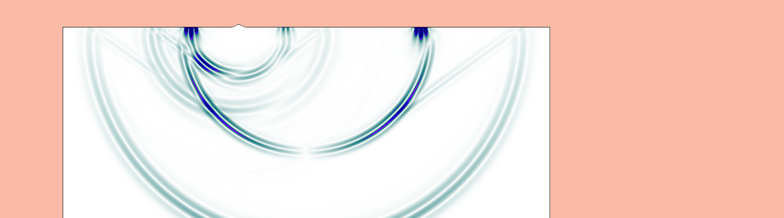
Animation of the propagation of the pressure wave in water and the immersed steel test sample.
Meshing and Solving
When meshing vibration problems, it is essential to spatially resolve the propagating waves in the structure. This is, of course, not specific to the dG time-explicit method, but applies to all wave-based physics of the Acoustics Module.
An important difference from wave problems solved in fluids (pressure acoustics) is that many different waves can propagate inside an elastic structure and at its surface. In the bulk, pressure (longitudinal) and shear (transverse) waves propagate. In the presence of a free surface or at an interface to another material, surface/interface waves can propagate; e.g., Rayleigh waves. One example is given in the image below. Yet further wave types are bending and torsional waves that propagate in waveguide configurations.
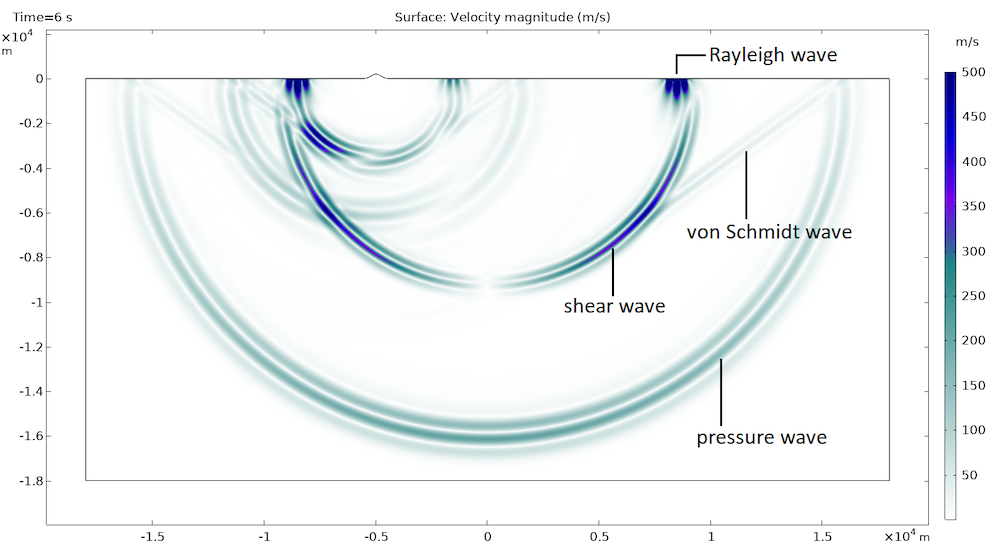
Propagation of four different waves in the Ground Motion After Seismic Event tutorial model.
The different waves propagate at different speeds and have different wavelengths. The slowest wave c_\textrm{min} has the shortest wavelength \lambda_\textrm{min}. This is the length scale that defines mesh size. The default for the Elastic Waves interface (as for the other time-explicit interfaces) is to use quartic (fourth-order) shape functions. This defines a Maximum element size as
where f_\textrm{max} is the maximal frequency component to be resolved in the propagating signal.
Notice that you only need about 1.5 mesh elements per wavelength to resolve the wave as quartic elements are used. It is always good practice to confirm that factor with a mesh convergence study. The computational mesh should, of course, also resolve geometric details and curved surfaces adequately. Typically, with the dG method, curved surfaces are well resolved by setting the Curvature factor to a value between 0.3 and 0.4. Remember that internally, COMSOL® uses higher-order mesh elements that curve.
As mentioned, the method described here uses a time-explicit time-stepping scheme. This sets a strict limit on the internal time step that the solver will take when stepping forward in time. The time step is controlled by the globally smallest value of the so-called cell wave time scale. The cell wave time scale is defined as the ratio between the local mesh size and the fastest wave that propagates, at speed c_\textrm{max}. This means that one small mesh element in a model will control the global time step that the solver can take. In most applications, the pressure waves propagate faster than the other type of waves, and hence the default is c_\textrm{max} = c_\textrm{p}, the pressure wave speed (this value can be changed when advanced physics options are turned on).
The cell wave time scale can be visualized by plotting the variable elte.wtc (turn off smoothing and refinement). The value does not directly represent the internal solver time step, but it allows the user to identify what elements are problematic and control the time step. Thus three considerations need to be taken into account when meshing a model solved with the Elastic Waves, Time Explicit interface:
- Resolve the smallest wavelength \lambda_\textrm{min} = c_\textrm{min}/f_\textrm{max} with about 1.5 elements.
- Resolve geometry details and curved surfaces.
- Generate a mesh that avoids small elements, if possible. A small value of the ratio between mesh size and fast wave speed c_\textrm{max} will dictate the time step.
These considerations are especially important when coupling domains that have different material properties (different speeds of sound). This can be in a multiphysics setting, coupling a fluid to a solid, or as a single-physics application when connecting solids with different material properties. You want to avoid a small mesh element defined by one set of material properties to propagate from one domain to the other. This happens when using conforming meshes in a union geometry (a geometry created by forming a union).
To remedy this, it is important to use a nonconforming mesh with an assembly geometry. For multiphysics applications, use the Pair Acoustic-Structure Boundary, Time Explicit multiphysics feature. When coupling solid domains with different material properties, use the Continuity condition found under the Pairs menu.
A union geometry is one geometry object composed of one or several geometry objects. In other words, it can contain interior boundaries that differentiate one domain or material from another. In an assembly geometry, all geometry objects, created up till the geometry finalization node, will be considered as disconnected in terms of physics. It is therefore important to connect the disconnected components using the aforementioned identity pairs and pair boundary conditions.
As an example, the cell wave time scale is plotted below for the Immersion Ultrasonic Testing Setup tutorial for the preferred assembly setup (left) and a union setup (right). The color scale is the same, but with the respective min/max values depicted. The assembly setup, with the nonconforming mesh, has a time scale minimum (2.93e-9) that is nearly twice that of the union setup (1.61e-9). This means that the assembly case will solve twice as fast and with fewer mesh elements.


Finally, the general guidelines about meshing discussed in the blog post “Using the Discontinuous Galerkin Method to Model Linear Ultrasound” also apply here. In 3D, it is important to enable the Element Quality Optimization that will optimize the mesh and try to avoid too small elements. In 2D, one option to generate a triangular mesh of uniform size is to first generate a mapped mesh and then transform it into triangles.
Note: For the time explicit methods, the constraints on the time step ensure stability of the method (if not met, the solution will grow exponentially and explode in the end). For the traditional FEM time-implicit-based interfaces, the solver is always stable. Here, using an appropriately tuned solver will ensure adequate numerical resolution in both time and space.
Postprocessing
When postprocessing results from the time-explicit interfaces, a few things should be kept in mind.
Because the default discretization order is quartic (fourth order), the automatically generated default plots use an element refinement set to 6. This setting should also be used when setting up more plots. If it is not set correctly, the results can look underresolved without being.
When solving large transient models, the stored data can become very important. To reduce storage, a good strategy is to only store data when and where needed, for example, on a boundary or in a few points. This is set up in Store fields in output, in the Values of Dependent Variables section in the solver settings. The Times requested in the Study Settings represent the output times where the solution is stored. Internally, the solver will take appropriate time steps.
These tips are also discussed in a previous blog post.
Tutorial Models
You can see the new interface used in the following models:
- Ground Motion After Seismic Event: Scattering off a Small Mountain
- Isotropic-Anisotropic Sample: Elastic Wave Propagation
- Angle Beam Nondestructive Testing
- Immersion Ultrasonic Testing Setup
Animated results from the Angle Beam Nondestructive Testing tutorial model.


Comments (18)
Robin James
June 2, 2020How can we find the directionally dependent displacement components u, v, and w in the material using this method for wave propagation problems?
Mads Herring Jensen
June 2, 2020 COMSOL EmployeeDear Robin, in comsol you can set up an extra equation that allows you to integrate the velocity field in time to get the displacement. This is, for example, shown in the tutorial model “Isotropic-Anisotropic Sample: Elastic Wave Propagation”. You can find a link to that model in the blog post. Best regards, Mads
Robin James
June 2, 2020Thank you so much for your response.
Will this also work for guided wave simulations or Lamb wave simulations?
Will the absorbing boundaries work well with anisotropic materials like multilayered composite laminates to remove all boundary reflections? How is this different from low absorbing boundary condition is the solid mechanics interface?
Mads Herring Jensen
June 17, 2020 COMSOL EmployeeDear Robin, the absorbing layer is not a boundary condition but a so-called sponge layer. It uses a combination of scaling, filtering, and the low absorbing boundary at the end to absorb remaining waves. The low absorbing boundary in solids can only absorb P and S waves, it is like a simple impedance condition in acoustics. The adsorbing boundary method is not directly transferable to classical FEM and implicit time schemes. With regards to anisotropic materials the absorbing layers also work, take, for example, a look at the model “Isotropic-Anisotropic Sample: Elastic Wave Propagation”. Best regards, Mads
Robin James
June 2, 2020I also see that from the Animated results from the Angle Beam Nondestructive Testing tutorial model (as displayed above on this page), there are a lot of reflections from within the wedge itself. how can one avoid these reflections?
Mads Herring Jensen
June 17, 2020 COMSOL EmployeeDear Robin, I think that all the reflections that you see in the animation and model are physical reflections, so they cannot be avoided. Best regards, Mads
Robin James
August 20, 2020Thanks for your response Mads! I look forward to your webinar next week.
yash kumar dhabi
August 30, 2020Hi Mads,
I recently attended your webinar for elastic waves in time domain. I was trying to rebuild the model by myself but I had a few questions:
1) When I tried to build the geometry, the identity pairs are not being defined automatically. Is that because I built it in a different way or something ?
Due to this, I am not able to define an absorbing layer and not able to do the next steps of the model.
2) The error that I am getting is below :
Compile Equations: Time Dependent (sol1/st1)
Error in multiphysics compilation.
Illegal domain selection.
– Pair: p1
Could you please guide me further ?
Thank you,
Yash
Mads Herring Jensen
August 31, 2020 COMSOL EmployeeDear Yash
The absorbing layers have nothing to do with the pair features. You can have a look at one of the tutorial models mentioned in the blog post to see how they are set up. The layer feature should be used when creating the geometry. When creating the geometry, and you need to create an assembly (two different materials), then in the last step of the geometry change the action from Form Union to Form Assembly. This will also automatically create the Identity Pair.
Best regards
Mads
Syed Ali
October 12, 2020Hi Mads,
I have a simple question regarding “Immersion Ultrasonic Testing setup” available in COMSOL Multiphysics.
Ideally, the amplitude of “Front-face reflected signal” should be less than the “Incident signal” right but in simulations the Front face reflected signal has higher amplitude compared to the incident signal. Any theory behind this phenomenon?
My understanding is that:
Incident signal = reflected signal + loss of signal in water + loss of signal in test sample.
Mads Herring Jensen
October 28, 2020 COMSOL EmployeeHi Syed,
You are right. I believe that what you see is due to two effects:
1) The less important maybe: edge effects (diffraction) from the source face. In this tutorial the transducer is modeled as having a uniform “piston” displacement this generates waves that travel from the edges (see the animation). The reflections are included when averaging the pressure over the transducer surface.
2) The source is modeled with a velocity condition, and the average pressure on the surface is averaged. When the wave reflects and interacts with the source you will get a “pressure doubling” as the wave interacts with its reflection.
So this is a tutorial where the transducer is modeled in a very simplistic manner.
Mohammed Adam
November 27, 2021Dear Sir, I want to write a code that shows the behavior of the seismic wave in the case of a cavitation layer in the ground at a depth of 2 meters.
jean michel Puybouffat
December 30, 2021I am very interesting about this topic , i need support to develope application foe Phase array linear or 2D
Konrad Juethner
December 22, 2022Does the Elastic Wave, Time Explicit application mode couple with the heat equation to model the thermoelastic wave in a structure that is produced by a short-duration and high-energy pulse?
Mads Herring Jensen
December 22, 2022 COMSOL EmployeeDear Konrad,
The time explicit formulation is not coupled to heat transfer, but we do have an implicit FEM based multiphysics interface, called thermoelasticity, that may be what you are looking for. The formulation exists for both time domain and frequency domain (harmonic) analysis.
Best regards
Mads
Wen Luo
March 16, 2023Hi Mads,
Would be grateful if you can kindly help me on the following:
(1) In the tutorial Isotropic-Anisotropic Sample: Elastic Wave Propagation, how do you determine the parameter Source Extent (dS)?
(2) in 3D, when I tried to use ‘Midsurface’ in Geometry to create a mid surface, which can be used as boundary, for Block, it showed Failed to identify offset faces. Then how can I create a mid surface for Block in 3D? This surface will be used to generate the seismic source via Gaussian function .
thanks,
Wen
Mads Herring Jensen
March 28, 2023 COMSOL EmployeeDear Wen
The source parameter extend dS is of the order of the mesh size, it cannot be smaller as we need to ensure that there are integration points in the region of the source definition. The reason is that we do not have point sources available in the interface. For point 2, please contact support.
Best regards,
Mads
yaochong sun
April 20, 2023In the “Ground Motion After Seismic Event”, the source is a force source and it adds the source time function to the velocity components. However, the seismic source of a real earthquake is a moement tensor source, which adds source time functions to the stress components. However, I did not find where to add source time functions to the stress components. Do you know how to implement the moment tensor? Thank you!