When designing bandpass-filter type high-Q devices with the finite element method in the frequency domain, you will likely come across a situation where you need to apply many frequency samples to more accurately describe the passband. Simulation time is directly proportional to the number of frequencies included in the simulation of a microwave device, with the time increasing as the frequency resolution used becomes finer. Two powerful simulation methods in the RF Module help accelerate the modeling of such devices.
A Brief Introduction to the Two RF Simulation Methods
The two simulation methods that we will discuss in today’s blog post are the asymptotic waveform evaluation (AWE) and frequency-domain modal methods. Both are designed to help you overcome the conventional issue of a longer simulation time when using a very fine frequency resolution or running a very wide band simulation. The AWE is quite efficient when it comes to describing smooth frequency responses with a single resonance or no resonance at all. The frequency-domain modal method, meanwhile, is useful for quickly analyzing multistage filters or filters of a high number of elements that have multiple resonances in a target passband.
Asymptotic Waveform Evaluation Method Fosters Reduced-Order Modeling
For our purposes, it would be too technical to talk about the numerical characteristics of the asymptotic waveform evaluation (AWE) — a reduced-order modeling technique. Instead, we will go over how to use this method in the RF Module. The solver performs fast-frequency adaptive sweeping using an AWE that is configured in the Frequency Domain study settings, shown below.
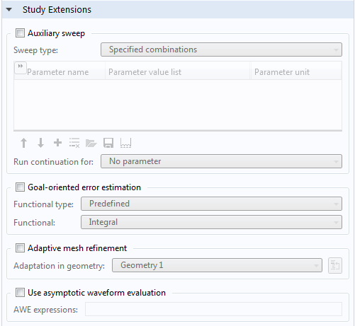
Study Extensions section of Frequency Domain study settings.
When the Use asymptotic waveform evaluation check box is selected, it will trigger an AWE solver. By default, the solver uses Padé approximations.
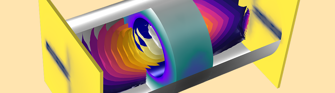
The AWE method is very useful when simulating resonant circuits, especially bandpass-filter type devices with many frequency points. For instance, the Evanescent Mode Cylindrical Cavity Filter tutorial model, available in the Application Library, sweeps the simulation frequency between 3.45 GHz and 3.61 GHz with a 5 MHz frequency step.


The Evanescent Mode Cylindrical Cavity Filter tutorial model (left) and its discrete frequency sweep results (right). The S-parameter plot does not look smooth around the resonant frequency.
Say you run the simulation again with a much finer frequency resolution, such as a 100 kHz frequency step that is 50 times finer. You can expect that the simulation will take 50 times longer to finish. When using the AWE option in this particular example model, the simulation time is almost the same as the regular frequency sweep case, but we can obtain all of the computed solutions on the dependent variable with the 100 kHz frequency step.
The simulation time also varies with regards to the user input in the AWE expressions. Any model variable works as an AWE expression, so long as it generates a smooth resulting plot like a Gaussian pulse or a smooth curve as a function of frequency. The absolute value of S21 (abs(comp1.emw.S21)), for example, works as the input for the AWE expression in the case of a two-port bandpass filter. For one-port devices like antennas, S11 still works. If the frequency response of the AWE expression contains an infinite gradient — the case for the S11 value of an antenna, with excellent impedance matching at a single frequency point — the simulation will take longer to complete. If the loss from the antenna is negligible, an alternative expression such as sqrt(1-abs(comp1.emw.S11)^2) may work well and reduce the computation time.
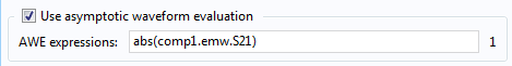
AWE expression using S-parameters (S21) for a two-port filter simulation.
Following the 100 kHz frequency step simulation, the solutions contain a ton of data. As a result, the model file size will increase tremendously when it is saved. When only S-parameters are of interest, a common theme in most passive RF and microwave device designs, it is not necessary to store all of the field solutions. By selecting the Store fields in output check box in the Values of Dependent Variables section, we can control the part of the model on which the computed solution is saved. We only add the selection containing these boundaries where the S-parameters are calculated. The lumped port size is typically very small compared to the entire modeling domain, and the saved file size with the AWE is more or less that of the regular discrete frequency sweep model when only the solutions on the port boundaries are stored.
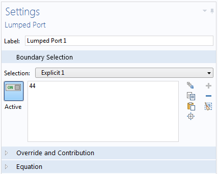
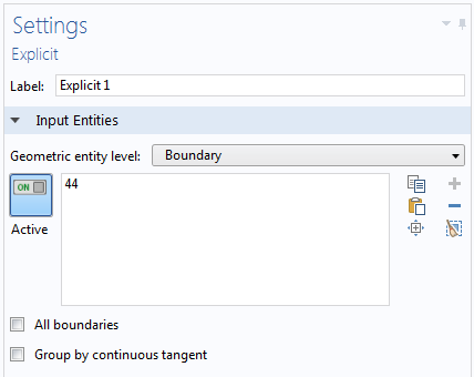
Settings window for the lumped port boundary (left) and the explicit selection generated by the lumped port (right).
It is easy to add an explicit selection when setting up the lumped port. When you specify the lumped port boundary selection, click the Create Selection button. This will add an explicit selection with the boundary you just added for the lumped port. By repeating the same step for the other port, you will obtain all of the selections to use for storing only those results that you need to plot the S-parameters.
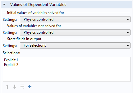
Values of Dependent Variables section of the Frequency Domain study settings.
In the Values of Dependent Variables section, change the selection in the Store fields in output combo box from All to For selections. You can then add the explicit selections created from the lumped ports.
Now you are ready to run the AWE frequency sweep. Don’t forget to use the finer frequency step in the study settings. You can do so in one of two ways: Directly type in the step you want, or click the Range button next to the input field to use the Range dialog box.
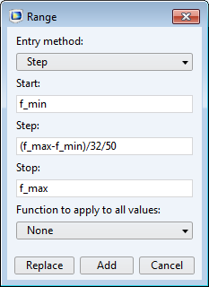
Updating the simulation frequency step via the Range dialog box.
Once the simulation is complete, you will notice that the simulation time for the AWE frequency sweep with a much finer step is almost the same as the discrete sweep. Let’s compare the computed S-parameters. Since the AWE performed a frequency sweep that was 50 times finer, its frequency response (S-parameters) plot consequently looks much nicer. Not only do you save precious time with this approach, but as the plot below illustrates, you also still obtain accurate and good-looking results.
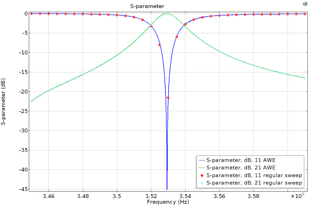
S-parameter plot of the AWE and discrete frequency sweep simulations.
Frequency-Domain Modal Method Captures the Resonance of Circuits
Bandpass-frequency responses of a passive circuit result from a combination of multiple resonances. Eigenfrequency analysis is key to capturing the resonance frequencies of an arbitrary shape of a device. Once we obtain all of the necessary information from the eigenfrequency analysis, we can reuse it in the frequency-domain modal study. Doing so enables us to optimize the efficiency of the simulation when a finer frequency resolution is required to more accurately describe the frequency response, as illustrated in the AWE method.
To perform a frequency-domain modal analysis seamlessly, there is one important simulation step to keep in mind. This step involves refining the eigenfrequency study results. The output of the eigenfrequency study is purely numerical and even includes nonphysical results. By using the manual eigenfrequency searching method, those unwanted, low-frequency residues can be filtered out. The manual eigenfrequency searching process is constrained by a series of items: Eigenfrequency search method around shift, Desired number of eigenfrequencies, and Search for eigenfrequencies around. For the last item, the lowest passband frequency works as a ballpark value.
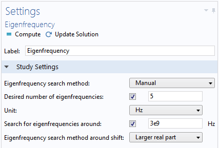
Manual search method in the Eigenfrequency settings.
To try this out, let’s take a look at the Coupled Line Filter tutorial model, available in our Application Library. You’ll want to add a new study with the eigenfrequency and frequency-domain modal study steps, configuring the settings for each study step as described above. Repeat this again with a frequency step that is 50 times finer. The Store fields in output check box in the Values of Dependent Variables section can also be applied to the frequency-domain modal study — if you are interested only in S-parameters, this is the way to go. By storing solutions only on the lumped port boundary, it is possible to further reduce simulation time.
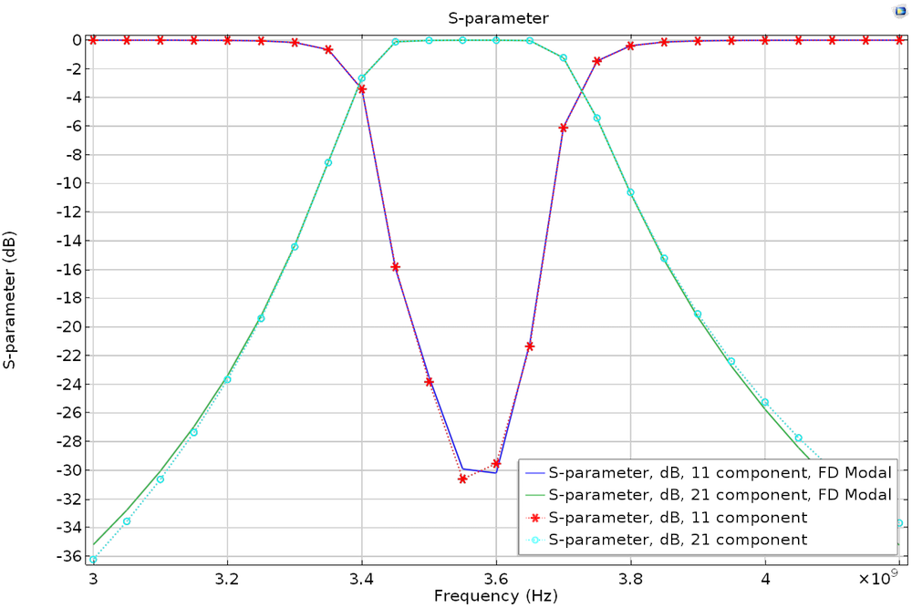
S-parameter plot of the regular frequency sweep and frequency-domain modal simulations.
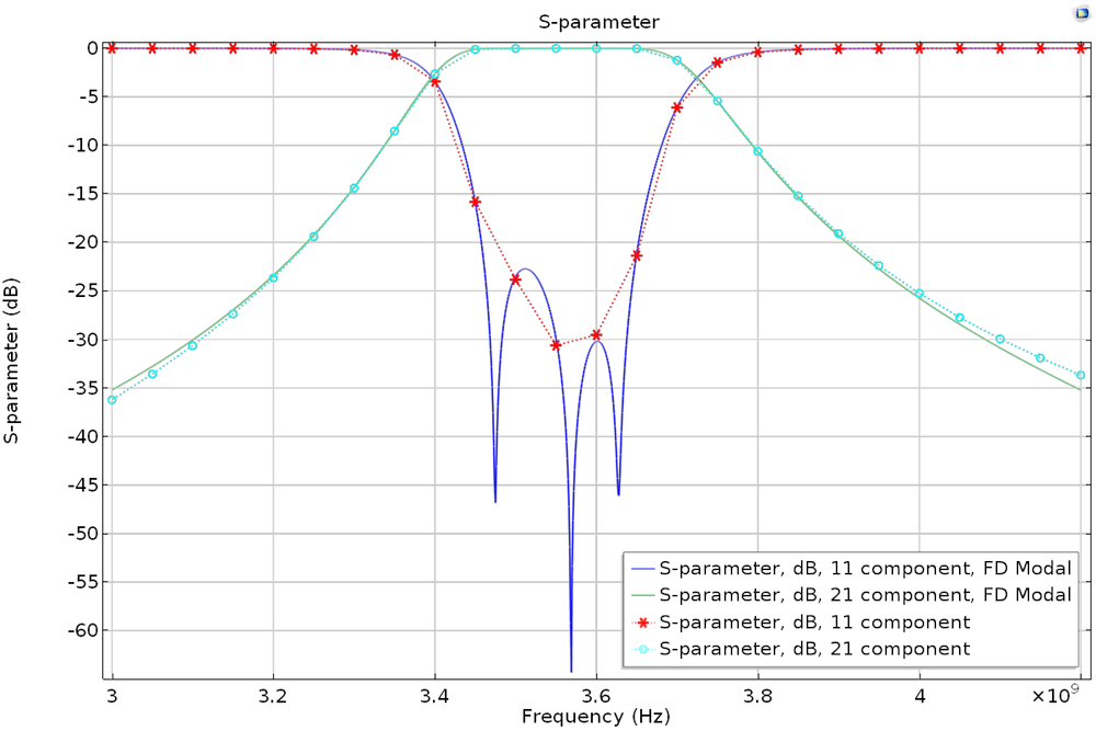
S-parameter plot of the regular frequency sweep and frequency-domain modal simulations with a frequency step that is 50 times finer.
Note that the eigenfrequency analysis contains a lumped port that impacts the simulation as an extra loading factor, so the phase of the computed S-parameters is different from that of the regular frequency sweep model. The results are compatible only with phase-independent S-parameter values such as dB-scaled, absolute value, reflectivity, or transmittivity.
Application Library Examples Now Available in COMSOL Multiphysics® Version 5.2a
The simulation methods presented in today’s blog post are powerful tools for enabling faster, more efficient modeling of passive RF and microwave devices. While these methods have been available since version 5.2, our latest release — COMSOL Multiphysics® version 5.2a — features polished Application Library examples that help further guide you in how to utilize these techniques. You can find such examples highlighted below:
- Asymptotic Waveform Evaluation method
- RF Module > Passive Devices > cylindrical cavity filter evanescent
- Frequency-Domain Modal method
- RF Module > Passive Devices > cascaded cavity filter
- RF Module > Passive Devices > coupled line filter
- RF Module > Passive Devices > cpw bandpass filter
Interested in learning about other improvements and upgrades in version 5.2a? Head over to our Release Highlights page for additional details.

Comments (0)