
Electrical cables are classified by parameters such as impedance and power attenuation. In this blog post, we consider a case for which analytic solutions exist: a coaxial cable. We will show you how to compute the cable parameters from a COMSOL Multiphysics simulation of the electromagnetic fields. Once we understand how this is done for a coaxial cable, we can then compute these parameters for an arbitrary type of transmission line or cable.
Design Considerations for Electrical Cables
Electrical cables, also called transmission lines, are used everywhere in the modern world to transmit both power and data. If you are reading this on a cell phone or tablet computer that is “wireless”, there are still transmission lines within it connecting the various electrical components together. When you return home this evening, you will likely plug your device into a power cable to charge it.
Various transmission lines range from the small, such as coplanar waveguides on a printed circuit board (PCB), to the very large, like high voltage power lines. They also need to function in a variety of situations and conditions, from transatlantic telegraph cables to wiring in spacecraft, as shown in the image below. Transmission lines must be specially designed to ensure that they function appropriately in their environments, and may also be subject to further design goals, including required mechanical strength and weight minimization.
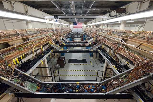
Transmission wires in the payload bay of the OV-095 at the Shuttle Avionics Integration Laboratory (SAIL).
When designing and using cables, engineers often refer to parameters per unit length for the series resistance (R), series inductance (L), shunt capacitance (C), and shunt conductance (G). These parameters can then be used to calculate cable performance, characteristic impedance, and propagation losses. It is important to keep in mind that these parameters come from the electromagnetic field solutions to Maxwell’s equations. We can use COMSOL Multiphysics to solve for the electromagnetic fields, as well as consider multiphysics effects to see how the cable parameters and performance change under different loads and environmental conditions. This could then be converted into an easy-to-use app, like this example that calculates the parameters for commonly used transmission lines.
Here, we examine a coaxial cable — a fundamental problem that is often covered in a standard curriculum for microwave engineering or transmission lines. The coaxial cable is so fundamental that Oliver Heaviside patented it in 1880, just a few years after Maxwell published his famous equations. For the students of scientific history, this is the same Oliver Heaviside who formulated Maxwell’s equations in the vector form that we are familiar with today; first used the term “impedance”; and helped develop transmission line theory.
Analytical Results for a Coaxial Cable
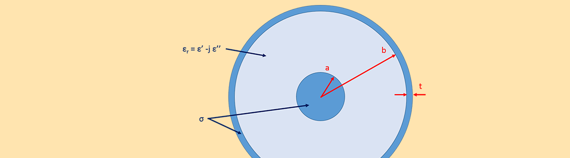
Let us begin by considering a coaxial cable with dimensions as shown in the cross-sectional sketch below. The dielectric core between the inner and outer conductors has a relative permittivity (\epsilon_r = \epsilon' -j\epsilon'') of 2.25 – j*0.01, a relative permeability (\mu_r) of 1, and a conductivity of zero, while the inner and outer conductors have a conductivity (\sigma) of 5.98e7 S/m.
The 2D cross section of the coaxial cable, where we have chosen a = 0.405 mm, b = 1.45 mm, and t = 0.1 mm. Note that this tutorial model is available for download in our Application Gallery.
A standard method for solving transmission lines is to assume that the electric fields will oscillate and attenuate in the direction of propagation, while the cross-sectional profile of the fields will remain unchanged. If we then find a valid solution, uniqueness theorems ensure that the solution we have found is correct. Mathematically, this is equivalent to solving Maxwell’s equations using an ansatz of the form \mathbf{E}\left(x,y,z\right) = \mathbf{\tilde{E}}\left(x,y\right)e^{-\gamma z}, where (\gamma = \alpha + j\beta) is the complex propagation constant and \alpha and \beta are the attenuation and propagation constants, respectively. In cylindrical coordinates for a coaxial cable, this results in the well-known field solution of
\mathbf{E}&= \frac{V_0\hat{r}}{rln(b/a)}e^{-\gamma z}\\
\mathbf{H}&= \frac{I_0\hat{\phi}}{2\pi r}e^{-\gamma z}
\end{align}
which then yields the parameters per unit length of
L& = \frac{\mu_0\mu_r}{2\pi}ln\frac{b}{a} + \frac{\mu_0\mu_r\delta}{4\pi}(\frac{1}{a}+\frac{1}{b})\\
C& = \frac{2\pi\epsilon_0\epsilon'}{ln(b/a)}\\
R& = \frac{R_s}{2\pi}(\frac{1}{a}+\frac{1}{b})\\
G& = \frac{2\pi\omega\epsilon_0\epsilon''}{ln(b/a)}
\end{align}
where R_s = 1/\sigma\delta is the sheet resistance and \delta = \sqrt{2/\mu_0\mu_r\omega\sigma} is the skin depth.
While the equations for capacitance and shunt conductance are valid at any frequency, it is extremely important to point out that the equations for the resistance and inductance depend on the skin depth and are therefore only valid at frequencies where the skin depth is much smaller than the physical thickness of the conductor. This is also why the second term in the inductance equation, called the internal inductance, may be unfamiliar to some readers, as it can be neglected when the metal is treated as a perfect conductor. The term represents inductance due to the penetration of the magnetic field into a metal of finite conductivity and is negligible at sufficiently high frequencies. (The term can also be expressed as L_{Internal} = R/\omega.)
For further comparison, we can compute the DC resistance directly from the conductivity and cross-sectional area of the metal. The analytical equation for the DC inductance is a little more involved, and so we quote it here for reference.
Now that we have values for C and G at all frequencies, DC values for R and L, and asymptotic values for their high-frequency behavior, we have excellent benchmarks for our computational results.
Simulating Cables with the AC/DC Module
When setting up any numerical simulation, it is important to consider whether or not symmetry can be used to reduce the model size and increase the computational speed. As we saw earlier, the exact solution will be of the form \mathbf{E}\left(x,y,z\right) = \mathbf{\tilde{E}}\left(x,y\right)e^{-\gamma z}. Because the spatial variation of interest is primarily in the xy-plane, we just want to simulate a 2D cross section of the cable. One issue, however, is that the 2D governing equations used in the AC/DC Module assume that the fields are invariant in the out-of-plane direction. This means that we will not be able to capture the variation of the ansatz in a single 2D AC/DC simulation. We can find the variation with two simulations, though! This is because the series resistance and inductance depend on the current and energy stored in the magnetic fields, while the shunt conductance and capacitance depend on the energy in the electric field. Let’s take a closer look.
Distributed Parameters for Shunt Conductance and Capacitance
Since the shunt conductance and capacitance can be calculated from the electric fields, we begin by using the Electric Currents interface.
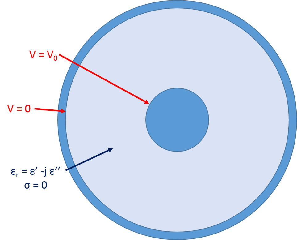
Boundary conditions and material properties for the Electric Currents interface simulation.
Once the geometry and material properties are assigned, we assume that the conductors are equipotential (a safe assumption, since the conductivity difference between the conductor and the dielectric will generally be near 20 orders of magnitude) and set up the physics by applying V0 to the inner conductor and grounding the outer conductor to solve for the electric potential in the dielectric. The above analytical equation for capacitance comes from the following more general equations
W_e& = \frac{1}{4}\int_{S}{}\mathbf{E}\cdot \mathbf{D^\ast}d\mathbf{S}\\
W_e& = \frac{C|V_0|^2}{4}\\
C& = \frac{1}{|V_0|^2}\int_{S}{}\mathbf{E}\cdot \mathbf{D^\ast}d\mathbf{S}
\end{align}
where the first equation is from electromagnetic theory and the second from circuit theory.
The first and second equations are combined to obtain the third equation. By inserting the known fields from above, we obtain the previous analytical result for C in a coaxial cable. More generally, these equations provide us with a method for obtaining the capacitance from the fields for any cable. From the simulation, we can compute the integral of the electric energy density, which gives us a capacitance of 98.142 pF/m and matches with theory. Since G and C are related by the equation
we now have two of the four parameters.
At this point, it is also worth reiterating that we have assumed that the conductivity of the dielectric region is zero. This is typically done in the textbook derivation, and we have maintained that convention here because it does not significantly impact the physics — unlike our inclusion of the internal inductance term discussed earlier. Many dielectric core materials do have a nonzero conductivity and that can be accounted for in simulation by simply updating the material properties. To ensure that proper matching with theory is maintained, the appropriate derivations would need to be updated as well.
Distributed Parameters for Series Resistance and Inductance
In a similar fashion, the series resistance and inductance can be calculated through simulation using the AC/DC Module’s Magnetic Fields interface. The simulation setup is straightforward, as demonstrated in the figure below.
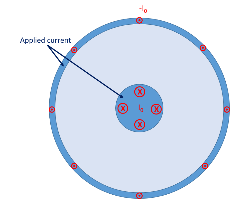
The center and outer conductor domains are excited with currents of equal magnitude and opposing directions, as indicated by the dots and crosses. The modeling features used for this purpose will allow for the current in the conductors to distribute freely according to skin and proximity effects, as opposed to the arbitrary distribution shown in the figure.
We refer to the following equations, which are the magnetic analog of the previous equations, to calculate the inductance.
W_m& = \frac{1}{4}\int_{S}{}\mathbf{B}\cdot \mathbf{H^\ast}d\mathbf{S}\\
W_m& = \frac{L|I_0|^2}{4}\\
L& = \frac{1}{|I_0|^2}\int_{S}{}\mathbf{B}\cdot \mathbf{H^\ast}d\mathbf{S}
\end{align}
To calculate the resistance, we use a slightly different technique. First, we integrate the resistive loss to determine the power dissipation per unit length. We can then use the familiar P = I_0^2R/2 to calculate the resistance. Since R and L vary with frequency, let’s take a look at the calculated values and the analytical solutions in the DC and high-frequency (HF) limit.

“Analytic (DC)” and “Analytic (HF)” refer to the analytical equations in the DC and high-frequency limits, respectively, which were discussed earlier. Note that these are both on log-log plots.
We can clearly see that the computed values transition smoothly from the DC solution at low frequencies to the high-frequency solution, which is valid when the skin depth is much smaller than the thickness of the conductor. We anticipate that the transition region will be approximately located where the skin depth and conductor thickness are within one order of magnitude. This range is 4.2e3 Hz to 4.2e7 Hz, which is exactly what we see in the results.
Characteristic Impedance and Propagation Constant
Now that we have completed the heavy lifting to calculate R, L, C, and G, there are two other significant parameters that can be determined. They are the characteristic impedance (Zc) and complex propagation constant (\gamma = \alpha + j\beta), where \alpha is the attenuation constant and \beta is the propagation constant.
Z_c& = \sqrt{\frac{(R+j\omega L)}{(G+j\omega C)}}\\
\gamma& = \sqrt{(R+j\omega L)(G+j\omega C)}
\end{align}
In the figure below, we see these values calculated using the analytical formulas for both the DC and high-frequency regime as well as the values determined from our simulation. We have also included a fourth line: the impedance calculated using COMSOL Multiphysics and the RF Module, which we will discuss shortly. As can be seen, our computations agree with the analytical solutions in their respective limits, as well as yielding the correct values through the transition region.
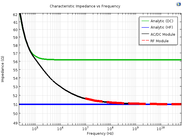
A comparison of the characteristic impedance, determined using the analytical equations and COMSOL Multiphysics. The analytical equations plotted are from the DC and high-frequency (HF) equations discussed earlier, while the COMSOL Multiphysics results use the AC/DC and RF Modules. For clarity, the width of the “RF Module” line has been intentionally increased.
Cable Simulation at Higher Frequencies
Electromagnetic energy travels as waves, which means that the frequency of operation and wavelength are inversely proportional. As we continue to solve at higher and higher frequencies, we need to be aware of the relative size of the wavelength and electrical size of the cable. As discussed in a previous blog post, we should switch from the AC/DC to RF Module at an electrical size of approximately λ/100. If we use the cable diameter as the electrical size and the speed of light inside the dielectric core of the cable, this yields a transition frequency of approximately 690 MHz.
At these higher frequencies, the cable is more appropriately treated as a waveguide and the cable excitation as a waveguide mode. Using waveguide terminology, the mode we have been examining is a special type of mode called TEM that can propagate at any frequency. When the cross section and wavelength are comparable, we also need to account for the possibility of higher-order modes. Unlike a TEM mode, most waveguide modes can only propagate above a characteristic cut-off frequency. Due to the cylindrical symmetry in our example model, there is an equation for the cut-off frequency of the first higher-order mode, which is a TE11 mode. This cut-off frequency is fc = 35.3 GHz, but even with the relatively simple geometry, the cut-off frequency comes from a transcendental equation that we will not examine further in this post.
So what does this cut-off frequency mean for our results? Above that frequency, the energy carried in the TEM mode that we are interested in has the potential to couple to the TE11 mode. In a perfect geometry, like we have simulated here, there will be no coupling. In the real world, however, any imperfections in the cable could cause mode coupling above the cut-off frequency. This could result from a number of sources, from fabrication tolerances to gradients in the material properties. Such a situation is often avoided by designing cables to operate below the cut-off frequency of higher-order modes so that only one mode can propagate. If that is of interest, you can also use COMSOL Multiphysics to simulate the coupling between higher-order modes, as with this Directional Coupler tutorial model (although beyond the scope of today’s post).
Mode Analysis in the RF and Wave Optics Modules
Simulation of higher-order modes is ideally suited for a Mode Analysis study using the RF or Wave Optics modules. This is because the governing equation is \mathbf{E}\left(x,y,z\right) = \mathbf{\tilde{E}}\left(x,y\right)e^{-\gamma z}, which is exactly the form that we are interested in. As a result, Mode Analysis will directly solve for the spatial field and complex propagation constant for a predefined number of modes. We can use the same geometry as before, except that we only need to simulate the dielectric core and can use an Impedance boundary condition for the metal conductor.

The results for the attenuation constant and effective mode index from a Mode Analysis. The analytic line in the left plot, “Attenuation Constant vs Frequency”, is computed using the same equations as the high-frequency (HF) lines used for comparison with the results of the AC/DC Module simulations. The analytic line in the right plot, “Effective Refractive Index vs Frequency”, is simply n = \sqrt{\epsilon_r\mu_r}. For clarity, the size of the “COMSOL — TEM” lines has been intentionally increased in both plots.
We can clearly see that the Mode Analysis results of the TEM mode match the analytic theory, and that the computed higher-order mode has its onset at the previously determined cut-off frequency. It is also incredibly convenient that the complex propagation constant is a direct output of this simulation and does not require calculations of R, L, C, and G. This is because \gamma is explicitly included and solved for in the Mode Analysis governing equation. These other parameters can be calculated for the TEM mode, if desired, and more information can be found in this demonstration in the Application Gallery. It is also worth pointing out that this same Mode Analysis technique can be used for dielectric waveguides, like fiber optics.
Concluding Remarks on Modeling Cables
At this point, we have thoroughly analyzed a coaxial cable. We have calculated the distributed parameters from the DC to high-frequency limit and examined the first higher-order mode. Importantly, the Mode Analysis results only depend on the geometry and material properties of the cable. The AC/DC results require the additional knowledge of how the cable is excited, but hopefully you know what you’re attaching your cable to! We used analytic theory solely to compare our simulation results against a well-known benchmark model. This means that the analysis could be extended to other cables, as well as coupled to multiphysics simulations that include temperature change and structural deformation.
For those of you who are interested in the fine details, here are a few extra points in the form of hypothetical questions.
- “Why didn’t you mention and/or plot all of the characteristic impedance and distributed parameters for the TE11 mode?”
- This is because only TEM modes have a uniquely defined voltage, current, and characteristic impedance. It is still possible to assign some of these values for higher-order modes, and this is discussed further in texts on transmission line theory and microwave engineering.
- “When I solve for modes using a Mode Analysis study, they are labeled by the value of their effective index. Where did TEM and TE11 come from?”
- These names come from the analytic theory and were used for convenience when discussing the results. This name assignment may not be possible for an arbitrary geometry, but what’s in a name? Would not a mode by any other name still carry electromagnetic energy (excluding nontunneling evanescent waves, of course)?
- “Why is there an extra factor of ½ in several of your calculations?”
- This comes up when solving electromagnetics in the frequency domain, notably when multiplying two complex quantities. When taking the time average, there is an extra factor of ½ as opposed to the equation in the time domain (or at DC). For more information, you can refer to a text on classical electromagnetics.
References
The following texts were referred to during the writing of this post and are excellent sources of additional information:
- Microwave Engineering, by David M. Pozar
- Foundations for Microwave Engineering, by Robert E. Collin
- Inductance Calculations, by Frederick W. Grover
- Classical Electrodynamics, by John D. Jackson

Comments (3)
Joohwa Lee
April 21, 2016This post is very interesting. Specially the impedance can be computed by either ACDC or RF modules. Is it possible to see model file(s) that generate the figure named ‘Characteristic impedance vs Frequency?’ I am interested in what models and boundary conditions to use. I think that potentials are given in ACDC. But what will be given in RF an how?
岩 李
July 2, 2018In the Magnetic Fields interface, how did you excite the current 1A and -1A? with lumped port or with coil?
Gabriel dos Santos
November 24, 2023Hello Andrew,
Very nice explanation.
I got a question when I read your blog.
What if I would like to obtain the R, L, C and G parameters as a function of frequency like you did in figure 6 for an underground cable or a subsea cable, how should I model the problem?
Of course, I need to model the water or de soil medium, but what boundary condition would be applied in the AC/DC model for it works in the high-frequency range (frequencies up to 1MHz). I tried to find some boundary condition like nabla times E = 0; however, I could not find it in the magnetic field module.
Any option to solve it using the AC/DC model?
Best regards,
Gabriel dos Santos