

A comprehensive set of functionality is available with the COMSOL Multiphysics® software to compute heat transfer in thin layers. A technical description of how this provides accurate results with minor computational effort could be the purpose of a full blog post and is not detailed here. Instead, we focus on the questions related to the Layered Material technology: What does it do? How does your simulation benefit from it?
Editor’s note: This blog post was originally published in 2019. It has since been updated to include new functionality available with the Heat Transfer Module as of version 5.5.
Modeling Heat Transfer in Thin Layers
COMSOL Multiphysics includes functionality that accounts for specific thermal properties in thin layers of a geometry and solves for heat transfer through layers without representing them explicitly in the geometry. Electric currents and mechanical stress can be defined in the layers for various fields of applications, such as electronic components and laminated composite shells exposed to thermal stress.
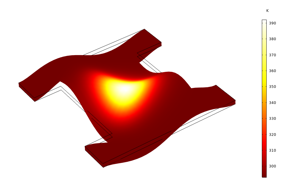
The image below shows the temperature distribution in a steel column subjected to a temperature gradient. A thin ceramic part made of two different layers, located at half-height of the column, acts as a thermal barrier due to its low thermal conductivity producing a jump in temperature across the ceramic part. The ceramic layer is represented as a surface in the geometry rather than two thin volumes to alleviate the constraint on the mesh size that would come with the high aspect ratio between the different parts of the geometry. This high aspect ratio would make the visualization in this part very difficult. Although the ceramic part is not represented explicitly in the geometry, you can solve the temperature distribution through the layer and magnify it for better postprocessing, as shown in the figure below.
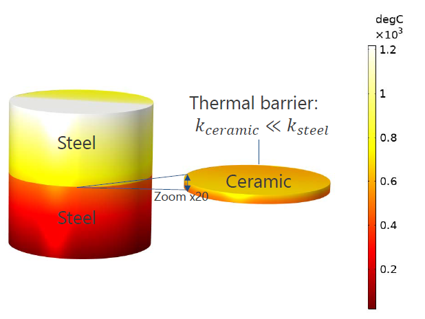
Temperature distribution in a steel column with a ceramic layer, computed with the Heat Transfer in Solids interface and the Thin Layer node. The thickness of the ceramic layer is enlarged 20 times for visualization.
See the Composite Thermal Barrier tutorial model in the Application Gallery for more details about this model.
What Does Layered Material Technology Bring to Heat Transfer Modeling?
The Layered Material technology is designed to improve your modeling experience in two ways:
- Grouping the definition of the layered shell’s properties in a central location in the model tree to make them accessible by the different physics interfaces involved. This is meant to clarify the model definition by separating the medium definition from the physics definition as well as to reduce the modeling work, since the medium properties are set once for all of the physics.
- Adding flexibility by allowing, for example, any number of layers or different positions and orientations for the layers.
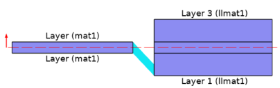
Let’s look at the design of the features for computing heat transfer in layered shells while taking advantage of the Layered Material technology. We consider an example geometry containing two layered shells:
- The first layered shell, defined on boundary 1, is composed of three layers made of material 1 (top and bottom) and material 2 (middle)
- The second layered shell, defined on boundary 2, is composed of a single layer made of material 3

Geometry containing the layered shells and material composition of the layered shells applied on boundaries 1 and 2.
The layered shells are included in the geometry as surfaces, but the physics equations can be solved on the reconstructed volume (shown in red in the figure below) with degrees of freedom (DOFs) added in the reconstructed volume.
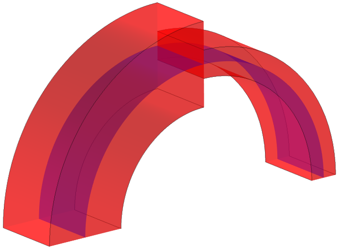
Reconstructed volume representation of the layered shells applied on boundaries 1 and 2 (10x scaling on the thickness).
When modeling heat transfer in this geometry, we want to specify the number of layers as well as the thickness and material of each layer. On top of these properties, it may be handy to have access to advanced parameters, such as the number of through-thickness mesh elements, orientation and position of the layered material on the boundary, and specific material properties at the interfaces of the layers.
All properties of layered shells, except the material, are defined by a Layered Material node. It includes the composition of the layered shell, along with the geometry and discretization properties of each layer. The physics node (Thin Layer for this example) simply points to the Layered Material node (middle part of the figure below). Then, the Layered Material node points to material nodes for the definition of the material properties (bottom part of the figure below).
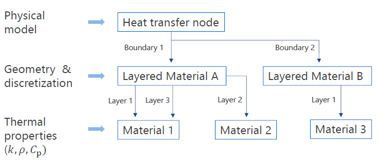
Model nodes involved in the definition of a layered shell.
Therefore, you can apply a single-physics model — let’s say, to model heat conduction — on several layered shells made of various numbers and types of layers. The specificity of the layered shells is handled by the Layered Material nodes. The modeling process is clarified by splitting the definition of the medium properties and physical model into two distinct locations in the model tree, as shown in the screenshot below:

Screenshot of the model tree and the Solid node Settings window.
Several layered material nodes are available:
- Single Layer Material
- Layered Material Link
- Layered Material Stack
- Layered Material
Read the blog post on analyzing wind turbine blades to see how these nodes can be combined to model a wind turbine composite blade.
Now that we’ve presented the functionality that comes with the Layered Material technology, two questions arise:
- How do we make use of this functionality for heat transfer?
- How does it benefit the simulation process?
Using the Layered Material Functionality in COMSOL Multiphysics®
In all versions of the Heat Transfer interface, the Thin Layer, Thin Film, and Fracture nodes can be used on boundaries to model layered shells made of solid, fluid, and porous materials (with any number of layers) using the Layered Material technology. The dedicated Heat Transfer in Shells interface, applicable on boundaries, allows the same modeling via its Solid, Fluid, and Porous Medium nodes and provides additional subnodes to account for layer heat sources and fluxes and continuity between layers, as described later in this post. (You can find details about these features in the Heat Transfer User Manual.)
Now, let’s clarify some of the settings that are available with the Layered Material technology. For this, we consider the Heat Transfer in Shells interface, which is applied on the example geometry mentioned in the previous section.
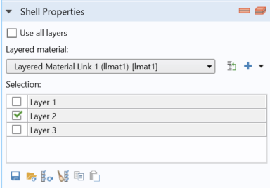
First, the Heat Transfer in Shells interface contains a Shell Properties section where the Shell type, Layered shell or Nonlayered shell, can be selected. The Nonlayered shell option switches to a simplified machinery that supports the simplest single layer shell configurations only. This lightweight option is of interest for the simplest physics and leads to a more responsible UI when the number of geometrical entities is very large. However, it does not provide the advanced pre- and postprocessing tools nor the multiphysics coupling capabilities available with the Layered shell option on which this post focuses. In the following part of this text, we will assume that the default Layered shell option is selected.
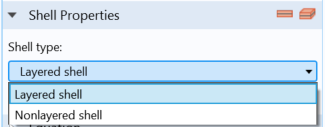
Screenshot showing the default Layered shell option selected in the Shell Properties section.
Because the layered shell properties are defined in the material nodes, the boundaries selected in the Heat Transfer in Shells node require a layered material defined on them. The Restrict to layered boundaries check box, located in the Boundary Selection section of the Heat Transfer in Shells interface, controls how the UI behaves depending on if layered materials are defined or not. When it is deselected (default option), it is possible to select any boundary. If no material — which is your configuration when you start to build the model — or a classical (nonlayered) material is defined on some of the selected boundaries, a red cross in the Materials node indicates that additional information is required.
So, with the Restrict to layered boundaries check box deselected, it is possible to go back and forth between the physics and the material definition, provided that everything is properly defined before the model is solved. Conversely, when the Restrict to layered boundaries check box is selected, only the boundaries where a layered material is defined can be selected. This automatically filters out the boundaries that are not shells, so the ones where it doesn’t make sense to define the Heat Transfer in Shells interface, provided the layered material properties have been properly defined before the physics is defined. From here, we’ll assume that the Restrict to layered boundaries check box is in its default state, deselected.
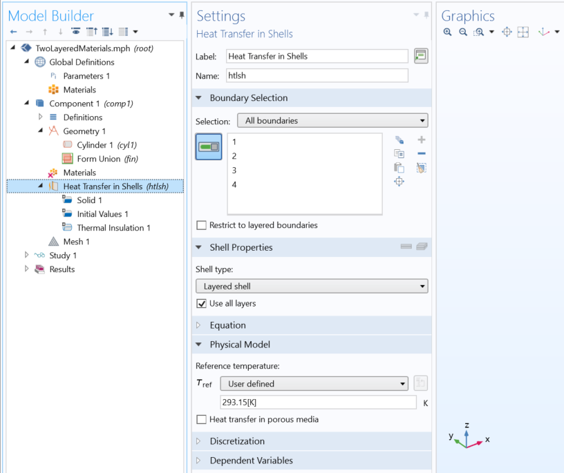
Screenshot showing the Heat Transfer in Shells interface Settings window with default options.
Single Layer Material
At this point, it is recommended to add layered materials under the Materials node. Let’s start with the simplest and most common configuration when modeling heat transfer, a simple shell made of a single layer.

Screenshot showing the creation of a layered material node under the Materials node.
We add a single layer material corresponding to the shell on Boundary 2, shown in the second figure at the beginning of this post. This node is similar to a classical material with, in addition to the classical material content, an Orientation and Position section and three extra material properties in the Material Contents section.
The Orientation and Position section contains the shell position and the coordinate system that gives the orientation in case of anisotropic properties.
The three additional material properties are Thickness, Rotation, and Mesh elements, which correspond respectively to the shell thickness; the in-plane rotation of the coordinate system — useful, for example, to change the material orientation in a parametric study; and the number of mesh elements that defines the through-thickness number of mesh elements for the layer discretization.
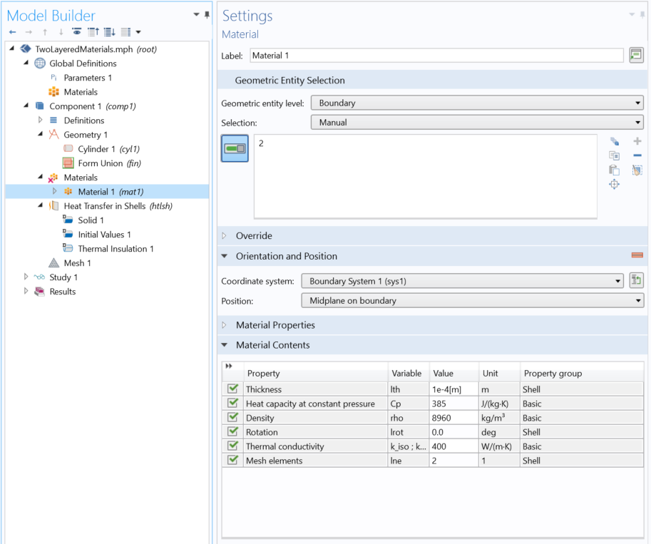
Screenshot showing the definition of a Single Layer Material node.
It’s interesting to note that if a material from a material library is added and assigned to a boundary where a layered material is expected, it is automatically converted into a Single Layer Material, with the Orientation and Position section appearing, along with the Thickness, Rotation, and Mesh elements material properties.
Layered Material
Let’s add a three-layer material corresponding to the shell on Boundary 1, shown in the second figure at the beginning of this post. Now, in the component, we add a Layered Material Link under the Material node. Similarly, to a Single Layer Material, we find the Orientation and Position section. The layer definition is linked to this node in the Layered Material Settings section, where it is possible to select any of the existing layered materials or create a new one using the + button. Depending on the type of layered material, different settings are available; see the Composite Material Module User Manual for details. In this example, we select a Layered Material.
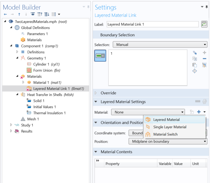
Screenshot of the Layered Material Link node where the + button is used to add a layered material.
The layered material is then created under the Global Definitions node. It is possible to define an arbitrary number of layers.
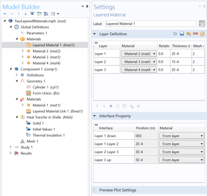
Screenshot of the Layered Material node defining a three-layer shell.
Each layer has its own link to a classical material that provides the layer material properties. In addition, the Rotation, Thickness, and Mesh elements are defined for each layer.
Extended Capabilities for Modeling Heat Transfer in Layered Shells
Once you’ve updated your model to use the Layered Material technology, flexibility is enhanced for several aspects of your simulation process. You can apply heat sources and fluxes on specific subsets of layers or at interfaces between layers (including the external interfaces), as illustrated below with the Heat Source and Heat Source, Interface nodes.
| Heat Source | Heat Source, Interface |
|---|---|
 /td> |
|
|
|
Screenshots of the Settings windows for the Heat Source (top left) and Heat Source, Interface nodes (top right) as well as the corresponding Layer Cross Section Preview images generated when clicking the buttons in the upper-right corners of the windows.
When considering thermal expansion, you can apply a rotation on each individual layer for the anisotropic modeling of heat transfer and solid mechanics. Another benefit is that specific through-thickness meshes can be used on layers, and you have the choice to set the temperature field as continuous or discontinuous at the common edge between adjacent layered shells (middle of the bow in the figure below); by default, it is continuous for thermally thin shells, otherwise it is discontinuous.
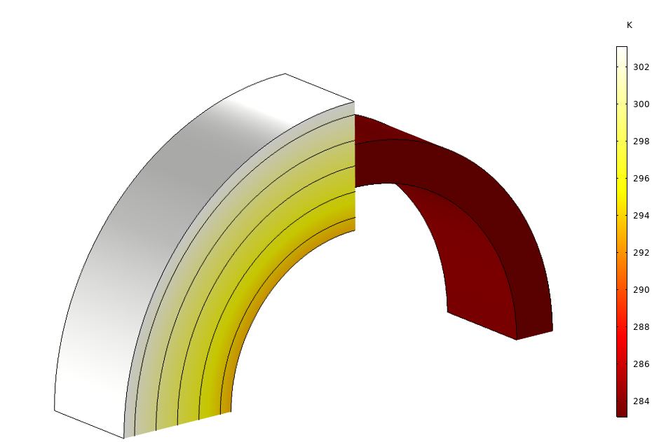
Temperature field, discontinuous at the edge where the layered materials coincide (10x scaling on the thickness).
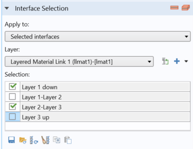
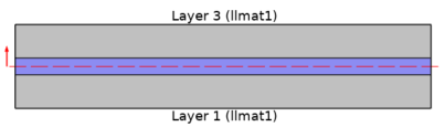
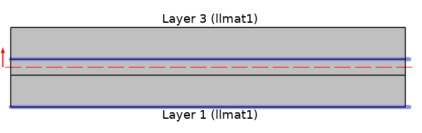
By using the Continuity node, the temperature continuity can be defined as needed, and it is possible to control the offset that defines the parts in contact, as shown below.
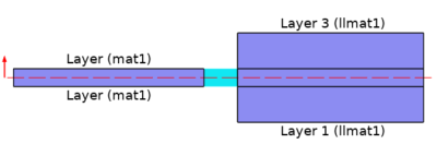
Layer Cross Section Preview of the Continuity node, applied between the layered materials of boundaries 1 and 2 with continuity on the bottom (left) or on the midplane (right).
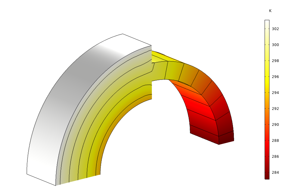
The temperature field, continuous at the edge where the layered materials coincide (10x scaling on the thickness), continuity defined on the midplane.
Several sketches to preview the layered material configuration are available for preprocessing, and specific plots allow you to visualize the computed fields through the thickness of the layered material; on slices of it; or on a full 3D representation (with scaling on thickness), as demonstrated above. More details about the Slice and Through thickness plots available with the Layered Material dataset can be found in this blog post on the Composite Materials Module.
Finally, for a greater numerical verification of the simulation results in a layered material, you can also evaluate layerwise averages and integrals by using specific operators. See the Composite Thermal Barrier tutorial model to get a demonstration of how the xdintopall operator can be set to integrate the temperature in the thermal barrier (in all layers), and how the atonly operator allows you to specify the evaluation context, for example, of a specific layer in the layered material. By combining these two operators, you can make sure the average temperature obtained in each layer with the thin layer approach is very close to those obtained when the thermal barrier is explicitly represented as a volume in the geometry.
Improving Performance by Making Assumptions on the Heat Transfer Pattern
Before concluding, we should review the different models available for heat transfer in layered shells (in the Thin Layer node, for example).
The most accurate model, the General option, implements the full heat transfer equations just like it is done for a domain. The discretization corresponds to the product of the boundary mesh and the number of mesh elements defined through the thickness of the layered material. Like the accuracy, the numerical cost is the same as for a meshed domain. The benefit of using this option is that it is not necessary to represent the geometry and mesh the actual layered structure: It is defined from a simple boundary and the layered material.
When the layers are considered either very good or very bad thermal conductors, two options with a lower numerical cost are available.
By using the Thermally thin approximation option, you assume thermal equilibrium between both sides of the layered shell. This applies well when the thermal conductivity of the layer is much higher than the conductivity of the surrounding material. The temperature gradient through the thickness of the layer can be neglected in comparison to the temperature gradients observable along the layer and in the surrounding geometry. With this option, only the shell contribution to the tangential heat transfer is accounted for, and the DOFs through the thickness of the layer are not included in the computation.
With the Thermally thick approximation option, it is the opposite configuration: because the layer is more thermally resistive than the surrounding material, the contribution of the shell to the gradient of temperature along the layered shell can be neglected. The heat flux across the layer is obtained by applying the thermal resistance to the temperature difference between both sides of the layer. In the Composite Thermal Barrier tutorial model, this approach produces reliable temperature predictions in terms of accuracy, when compared to the General option.
These approximations — associated to a Single Layer Material node when modeling one layer or applied to the layered shell when using other types of layered materials — help to improve the efficiency of the computation.
Concluding Thoughts
In this blog post, we have taken an in-depth look at the design of the thin layer functionality for heat transfer based on the Layered Material technology. You can access an extended set of functionality with improved preprocessing and postprocessing tools as well as flexibility in the simulation process for configurations of complex layers.
Other physics interfaces are designed to use the Layered Material technology as well. Multiphysics coupling nodes are available to model multiphysics processes such as thermal expansion, electromagnetic heating, and the thermoelectric effect in layered materials. For example, see the Thermal Expansion of a Laminated Composite Shell model in the Application Gallery.
Temperature distribution and deformation (scaled 200x) of a composite laminate made of 6 layers with various fiber orientations and subjected to narrow beam heating.
Further Reading
Read more about layered material technology on the COMSOL Blog:

Comments (5)
Jean-Marc Petit
April 1, 2019Great post !
Harek Tarek
May 16, 2020I want to receive all news
Robert Bedard
May 18, 2020An eye opener post. Heat transfer modeling through Layered shell is availble with the Heat transfer module, right? Is it included in the CFD module? Thanks!
anna Mathew
September 6, 2020Great post .
Jaramillo Diego
March 10, 2022The layered model example is available in the PDF version?