

When we analyze high-frequency electromagnetics problems using the finite element method (FEM), we often compute S-parameters in the frequency domain without reviewing the results in the complementary domain; that is, the time domain. The time domain is where we can find other useful information, such as time-domain reflectometry (TDR). In this blog post, we will demonstrate data conversion between two domains in order to efficiently obtain results in the desired computation domain through a fast Fourier transform (FFT) process.
Very Wide Frequency Range S-Parameter Calculation
Say you are simulating a device and want to get a very wideband frequency response with a small frequency step in the frequency domain or the time-domain reflectometry with a long time period. This would take a long time. However, in both cases, the computation performance in a wide range of frequencies and times can be boosted by running the simulation in the complementary domain first and then conducting a FFT to generate the results in the preferred domain. For example, you can:
- Simulate a transient analysis, and then run a time-to-frequency FFT for a wideband frequency response
- Perform a frequency sweep, and then a frequency-to-time FFT for a time domain bandpass impulse response
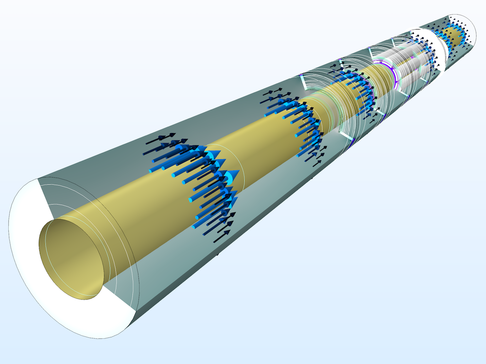
Logarithmic surface plot of the electric field norm and arrow plot of time-averaged power flow in a coaxial low-pass filter at 10 GHz.
Performing a wideband frequency sweep with a small frequency step size could be a time-consuming and cumbersome task. A sharp resolution of the frequency response of a device can be found from the time-to-frequency FFT, where the ending time of the transient input to the FFT process defines the frequency resolution of the final results.
Consider a modulated Gaussian pulse used for an excitation source to drive a time-domain model for a wideband response in the frequency domain. The excited energy gradually decays in general as time passes by, and it eventually vanishes. The longer the time-domain simulation is performed as an input to the FFT, the finer the frequency step size in the FFT output. When the amount of energy in the simulation domain is negligible after a certain time period, there is no need to continue the simulation. Instead, we can stop the transient simulation when the energy is less than a certain threshold and fill the solutions with zeros in the remaining time before executing the FFT. We call this process zero-padding.

The time-domain voltage at the excitation (source) lumped port. Left: The voltage is converging to zero and S-parameters are in the frequency domain. Right: Reflection property (S11) and insertion loss (S21) are plotted in a 60-GHz bandwidth.
Far-Field Radiation Pattern of Wideband and Multiband Antennas
A wideband antenna study, such as a S-parameter and/or far-field radiation pattern analysis, can be obtained by performing a transient simulation and a time-to-frequency FFT. We can run a time-dependent study first and then transform the dependent variable (magnetic vector potential A) to convert a voltage signal at a lumped port from the time domain to the frequency domain. S-parameters and far-field radiation results are computed from the converted frequency domain data. The following dual-band printed antenna shows two resonances, where the computed S11 is below -10 dB in the S-parameter plot for the given frequency range.
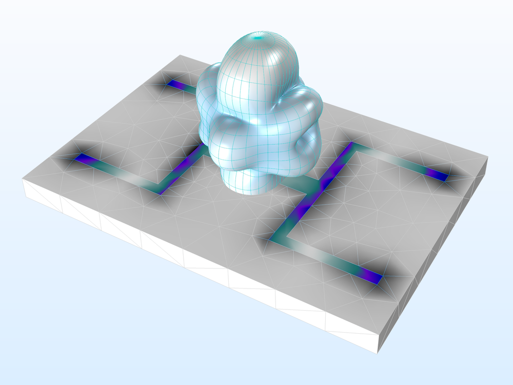
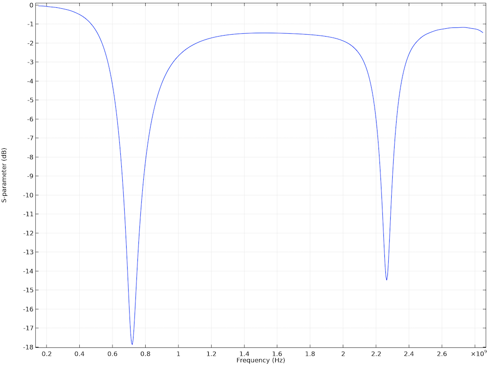
Left: Surface plot of the electric field norm and far-field radiation pattern of a dual-band printed strip antenna at 2.265 GHz. Right: S-parameter plot shows two resonance regions where the computed S11 is below -10 dB.
Two-Step Process with Time-to-Frequency Fourier Transform
In the Lumped Port Settings window, clicking the Calculate S-parameter check box on the excitation port sets the voltage excitation type to the modulated Gaussian. The center frequency (f0) of the modulating sinusoidal function can also be specified.
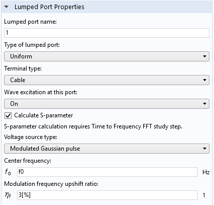
Lumped port settings in the Electromagnetic Waves, Transient physics interface.
The modulated Gaussian excitation voltage is defined as:
where \sigma is the standard deviation 1/2f0, f0 is the center frequency, and \eta_f is the modulating frequency shift ratio.
A small ratio value (for example, 3%) of \eta_f may enhance the frequency response around the highest frequency.
The frequency here has to be matched to the center frequency of the S-parameter calculation used in the time-to-frequency FFT study step from the Model Builder tree.


Left: Time-dependent study step settings. Center: Time-to-frequency FFT study step settings. Right: Default solver sequence in the Model Builder tree.
The end time of the time-dependent study step is set to 100 times that of the period of the modulating sinusoidal function, which could be long enough for a simple passive device to ensure that the input energy is fully decayed. This works for typical passive circuits, except for closed-cavity-type devices, where the energy decay time can be much longer.
The stop condition is automatically added under the time-dependent solver (the Calculate S-parameter check box activates this stop condition in the solver settings). When the sum of the total electric and magnetic energy in the modeling domain is less than 70 dB compared to the input energy, the time-dependent study is terminated by the stop condition and all time-domain data is passed to the FFT step. To generate the frequency-domain data without significant distortion in the frequency range between 0 and 2f0, the time step, satisfying the Nyquist criterion, is set to 1/4f0 = 1/2B, where B is the bandwidth 2f0.
To provide a fine frequency resolution, the end time of the FFT study step is much longer than that of the time-dependent study. Zero-padding is automatically applied to the time-dependent study data before the FFT study step.
Time Domain Bandpass Impulse Response of a Transmission Line
While transient analyses are useful for time-domain reflectometry (TDR) to handle signal integrity (SI) problems, many RF and microwave examples are addressed using frequency-domain simulations generating S-parameters. However, from the frequency-domain data, it is difficult to identify sources for this signal degradation.
By simulating a circuit in the frequency domain and performing a frequency-to-time FFT, a voltage signal in the frequency domain can be investigated in the time domain. The computed results can help identify the physical discontinuities and impedance mismatches on the transmission line by analyzing the signal fluctuation in the time domain.
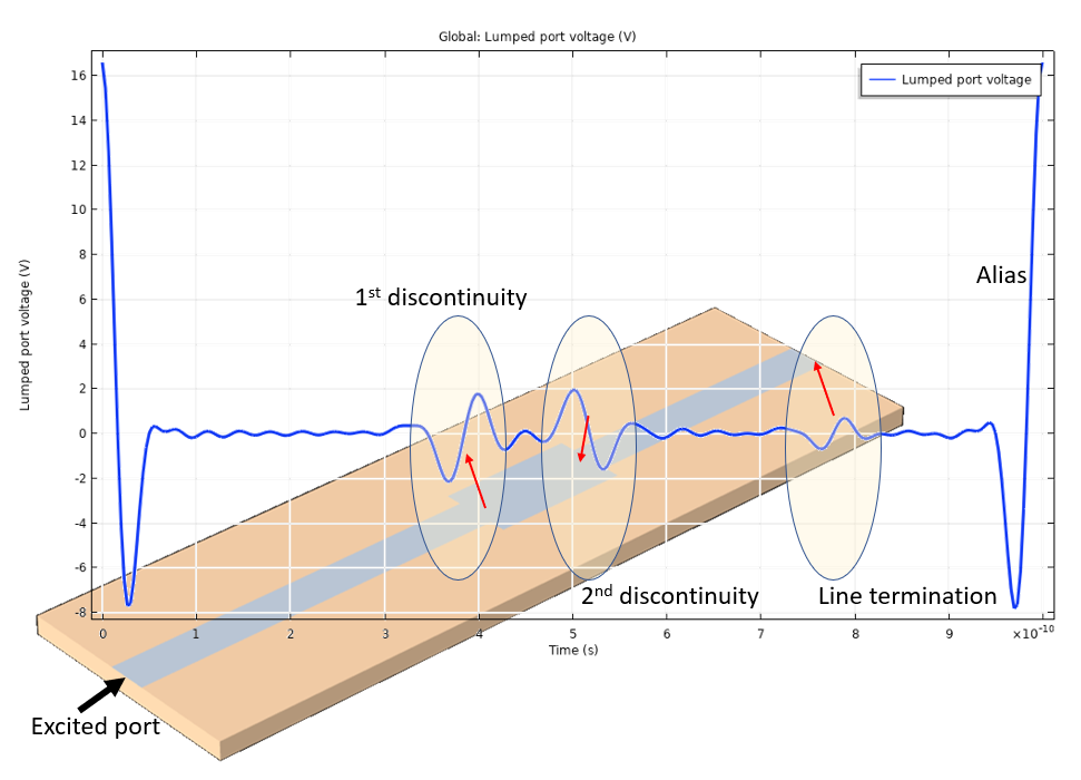
Time domain lumped port voltage. The overshoot and undershoot of the signal indicate the discontinuities of the microstrip line.
In the above figure, the time-domain results of the voltage bandpass impulse response at lumped port 1 are plotted with a microstrip line that has a couple of line discontinuities. The voltage fluctuation times correspond to the propagation times for the incident pulse to be reflected from the two line discontinuities: the defective parts of the 50-ohm microstrip line. The roundtrip travel time from lumped port 1 to each discontinuity agrees with the voltage fluctuation location.
Two-Step Process with Frequency-to-Time Fourier Transform
The time-domain results may vary with the input arguments in each study step. The impacts of the study step input arguments are described in the table below:
| Study Step | Argument | Impact on Transformed Time-Domain Result |
|---|---|---|
| Frequency domain | Start frequency | Low-frequency envelope noise |
| Stop frequency | Resolution and high-frequency ripple noise | |
| Frequency step | Alias period | |
| Frequency-to-time FFT | Stop time | Alias visibility |
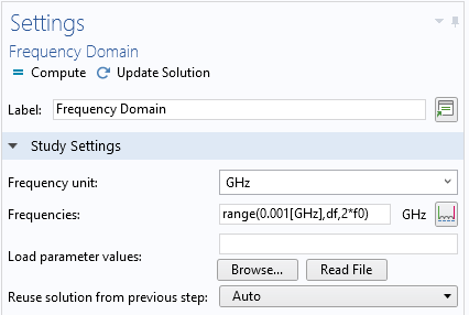
Frequency domain study step settings.
The frequency step, \Delta f (that is, df in the frequency domain study step settings above), is set to make the period of alias in the time-domain response greater than the roundtrip travel time from the excitation, lumped port 1, to the line termination, lumped port 2:
1/\Delta f = 1 ns > 2d\sqrt{\epsilon_r}/c_const
where d is the circuit board length; \epsilon_r is the permittivity; and c_const is a constant for the speed of light in vacuum, predefined in the COMSOL Multiphysics® software.
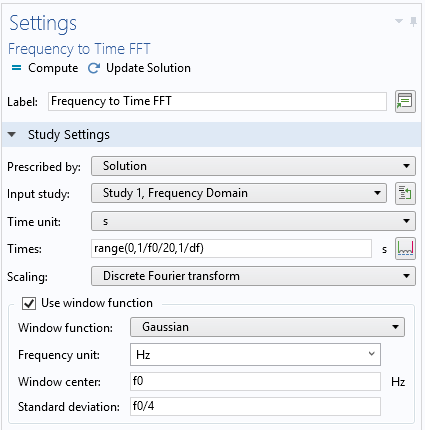
Frequency-to-time FFT study step settings.
While performing FFT, a Gaussian window function is used. This helps to suppress the noise coming from the limited range of the frequency sweep. Each study step uses the Store fields in output option, which defines the selections where the computed results are stored. By choosing only the lumped port boundaries for the Store fields in output settings, it is possible to greatly reduce the size of the model file.
Managing Computed Results
Since the FFT only transforms the dependent variable from the first domain, it is only possible to use postprocessing variables directly related to the dependent variable in the second domain. The first domain results are still accessible, typically through the Solution Store 1 data set.
The frequency-to-time FFT study step transforms the solution of the dependent variables in the frequency domain to the time domain with a very small time step of ten samples per period, defined by the highest frequency in the model. Only the postprocessing variables that can be expressed with the dependent variables are valid for results analysis. Since the transformed solutions typically contain many time steps, it is recommended to use the Store field in output option to reduce the size of the model.
Try These Application Examples of RF Signal Transformation
The simulation methods using fast Fourier transform presented in this blog post make RF and microwave device modeling more efficient. Try performing a time-to-frequency FFT for a wideband evaluation of S-parameters in this tutorial model of a coaxial cable:
Browse additional examples in the Application Library in the COMSOL® software:
- RF Module > Filters > coaxial_low_pass_filter_transient
- RF Module > Antennas > dual_band_antenna_transient
- RF Module > EMI_EMC_Applications > microstrip_line_discontinuity (Frequency-to-time for a quick investigation of TDR)


Comments (3)
SUNWOOK JUNG
November 23, 2018Thanks
Chen Guanren
August 8, 2019Thank you so much for the excellent instances and interpretation.
I’m now reproducing the template ‘Study of a Defective Microstrip Line via Frequency-to-Time FFT Analysis’ (microstrip_line_discontinuity, Application ID: 67361) in terms of the tutorial manual (models.rf.microstrip_line_discontinuity.pdf), and I hope that I can apply this method to our studies.
However, I encountered a problem during my reproduction. The latest version of COMSOL in our laboratory is 5.2a, then I tried to establish the model using it, by following the tutorial PDF step by step. Computation was run successfully, while the result in frequency domain remains to be zero over the whole frequency span, and the time-domain results were NaN. I checked the model over and over again, but still could not find where the problem is. The evaluation remains unchanged even though I added excitation in lumped port 1.
Is it possible that 5.2a can’t support this function perfectly, or some additional steps are needed for a correct computation?
I attached my reproduced 5.2a model here, could you please kindly have a look at it, and point where the problem is? I’d be very grateful if I can hear from you.
Best regards,
Chen
Reproduced model:
https://drive.google.com/file/d/1O5jXKibc7QQiUqgERp4BwIr5lJWUQhF4/view?usp=sharing
Mohammad Azadifar
December 16, 2020Very interesting case study, however the temw only support lumped port, hence one cannot analyse a multi pin configuration (which is essential for the analysis of high speed interconnects).
Furthermore, multipin configuration can be done in frequency domain, then using an ifft one may drive the time response. However the calculation over a broad range of frequencies can be really time consuming.
Moreover due to the trunction of response in high frequencies, early response to a step input will be really contaminated with ringing and one must modify the structure.
Is there any plan for an implementation of modal parameter estimation methods rather than an ifft?