

Continuing his discussion of simulation apps, guest blogger Mehrzad Tabatabaian presents an app that he designed to study transient heat transfer in a nonprismatic fin.
In earlier blog post, I spoke about my new book, COMSOL5 for Engineers, a resource designed to inspire and guide the creation of COMSOL models and simulation apps. Today, I’ll share a model with you that I created to analyze transient heat transfer in a fin as well as its corresponding app.
Transient Heat Transfer in Fins
One of the main functions of a fin — a thin component that is attached to a larger body — is to increase surface areas to optimize heat transfer. In this case, transient heat transfer is a combination of mechanisms based on conduction and convection. The fin begins by conducting heat through its solid domain and the surrounding air/fluid takes away the heat via convection, generally for cooling purposes. When the temperature does not change at any given point in the fin, with respect to time for a set of given boundary conditions, a steady state of equilibrium has been reached.
In many practical applications, the transient state is neglected due to the relatively short duration of time that is needed to reach the steady state. Some important modeling questions, however, still remain:
- What is the exact duration of time?
- What parameters are affecting this length of time?
The answers to these questions provide a better understanding of the physics involved and hence an improved fin design.
The example I’ll focus on today — which comes from my book COMSOL5 for Engineers — is of a fin, with circular cross sections, that is attached to a section of a wall. Let’s begin by looking at some of the underlying physics behind transient heat transfer as well as important design considerations in a fin.
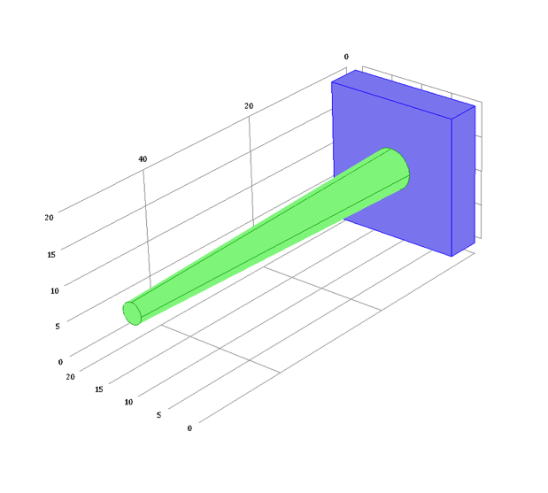
Geometry of a nonprismatic fin attached to a wall. The length of the fin (measured along its axis) is L, base-area radius is R_b, tip-area radius is R_t, and total heat transfer surface is A_{fin}.
Implementing the Physics of Transient Heat Transfer into a Fin Model
In transient heat transfer, the governing PDE is as follows:
where t is the time, \rho is the material density, C is the heat capacity, k_s is the thermal conductivity of the fin, T is the temperature, and Q is the heat source/sink per unit volume and time.
Two dimensionless numbers — the Biot number (B_i = hL_c/k_s) and Fourier number (F_0 = \alpha t / {L_c}^{2}) — are used to scale the unsteady heat transfer and nondimensionalize the governing equation. In these equations, \alpha is the thermal diffusivity, h is the heat transfer coefficient corresponding to the fin’s surface area, and L_c is the length scale. For a sphere, L_c is equal to 1/3 of its radius. For this fin example, L_c = A/p, with A representing the cross-sectional area and p representing a perimeter at a given section of the fin, say at a distance x from the wall and/or base.
For a fin, the medium tends to have a large aspect ratio, meaning that greater attention should be given to the definition of B_i. This is accomplished by distinguishing the radial direction of conduction from the axial direction. In the case of today’s example, for a small B_i as compared to unity, the temperature variation in the radial direction is negligible.
In the model, a material-based length scale is also defined: \ell = \frac{k_s}{h}. The ratio of the two length scales involved, or L_c / \ell, is actually another interpretation of B_i. For instance, when B_i < 1, the geometry-based length scale is insignificant in comparison to the property-based one and vice versa when B_i > 1. Their product,L_c \cdot \ell, gives a useful quantity in fin thermal analysis and design. It is defined here as L_c \cdot \ell = m^{-2}, where m = \sqrt{hp/k_sA}.
The dimensionless quantity mL, sometimes called the fin number, is an important design parameter that affects a fin’s overall performance and its physical meaning is significant to a fin’s thermal analysis. It can be interpreted as the ratio of conduction resistance in the axial direction to the gross external convection resistance. When mL is small, the temperature drop is small along the fin’s axis. When it is large, the temperature drop is also large and the fin’s tip temperature can asymptote to that of an ambient temperature T_{amb}.
For 1D steady-state heat transfer, with constant material properties and no heat source, the governing equation reduces to
The analytical solution for the 1D governing equation, as highlighted in Ref. 1, is relatively simple, as it is a linear combination of exponential functions. It is more challenging, but still possible, for transient cases with temperature-dependent, nonuniform material properties (see Ref. 2). Numerical solutions and/or design tables are typically used for the latter situation.
With the underlying physics of the model defined, I now have a tool that can be used by those with simulation expertise to test the performance of a fin. But what if I could take things a step further and make all of this complex underlying physics available in a simplified, intuitive format? The solution: Create an app.
Designing a Simulation App for a Cylindrical Fin
Apps, as I’ve previously noted, are powerful tools in the sense of design purposes as well as for educational aid. Today, I want to focus not so much on how to build this particular app but rather provide an example of its use.
To start, let’s first have a look at the app’s user interface (UI). As you can see, it includes a number of features and functionality that are designed to facilitate a good user experience. In the Input Parameters section, for example, modifications can easily be made to the fin’s geometrical dimensions as well its material properties. Selecting the Geometry & Mesh button provides a view of the fin in the graphics window, while choosing the Compute button produces further visualizations via simulation results for temperature contour or base/tip temperatures, to name a few possibilities. Perhaps you are interested in seeing how your simulation evolves over time. With the Animation button, you can easily visualize such elements. Such an animation could, for instance, show how the temperature along the fin’s axis changes over time.

The app’s user interface.
This leads us to a numerical example. Consider an aluminum fin that is 2 cm in diameter and 8 cm in length. The fin is attached to a wall at 150°C and has a thermal conductivity of 205 W/(m.K), with a heat transfer coefficient of 120 W/m2 at an ambient air temperature of 26°C. Using the app highlighted above, I’ll calculate the temperature profile of the fin and determine the tip temperature with/without heat transfer from the surface of the fin’s tip (in other words, insulated).
The screenshot below shows the app’s input parameters, along with the fin surface temperature variation results (after more than 150 s). The calculations give the following: mL = 0.8656. This indicates a relatively acceptable value for a design criteria of 1. In practice, a fin with mL \backsimeq 2 to 3 is considered to be sufficiently long.

Input parameters and surface temperature.
The tip temperatures are consistent with the expected drop in temperature from the base towards the tip. The temperature at the tip becomes steady after about 100 s at a value of around 110°C, as in the following figure. While an insulated tip was considered here, the app can also be used to obtain results for an uninsulated tip with a given heat transfer coefficient. The heat transfer ratio compared to a very long fin (i.e. T \approx T_{amb}) is, for steady state, tanh mL = tanh (0.8656) or 70%. With constant material properties, the analytical solution for steady state is given for the uninsulated tip as:
where \Theta = \frac{T -T_{amb}}{T_{wall} -T_{amb}} is dimensionless temperature.
Therefore, \Theta \mid _{x=L} is the tip temperature of T= 111.43°C. A similar analytical result for the insulated tip, \Theta = \frac{cosh \left(mL(1 -\frac{x}{L})\right)}{cosh (mL)}, gives T= 111.66°C. This data matches with the results from the app, which are also shown below — an indication of an app’s ability to balance accuracy with efficiency.
Reducing the radius of the fin can help improve its overall performance. With the app, users can easily verify that for a radius of 1 cm (instead of the original 2 cm), the tip temperature drops to about 90°C for an mL of 1.224.


Left: Base and tip temperature as a function of time for a radius of 2 cm. Right: Dimensionless temperature along the fin axis.
Apps Hide Complexity in a User-Friendly Interface
Today, I have discussed some of the underlying physics behind transient heat transfer in a fin design, while demonstrating how a complex model analyzing such physics can be turned into an easy-to-use app. With this tool, a greater number of people can run parametric analyses, from testing different fin geometries to different material properties, and thus achieve an optimal design more quickly. Note that the analytical solution, which can be complex, is available only for simple configurations; with temperature-dependent material properties or a variable radius, it is often impossible to find them.
What we have presented here is just one example of what you can create with the Application Builder. I encourage you to explore its many capabilities by starting to build apps of your own.
References
- Introduction to Heat Transfer, 6th Edition, Theodore L. Bergma, et. al., Wiley, 2011.
- Heat Conduction Using Green’s Functions, 2nd Edition (Series in Computational Methods and Physical Processes in Mechanics and Thermal Sciences), Kevin D. Cole, et. al., CRC Press, 2010.
- COMSOL5 for Engineers, M. Tabatabaian, Mercury Learning and Information, 2015.
About the Guest Author
Dr. Mehrzad Tabatabaian is a faculty member and the program head for the Mechanical Engineering Department, School of Energy at the British Columbia Institute of Technology (BCIT). Along with over fifteen years of teaching experience, Tabatabaian performs research on alternative energy systems and serves as the research committee chair for the School of Energy. He has authored several textbooks and published papers in scientific journals and at conferences, and he also holds several patents in the energy field, including fuel cell, wind, and solar power. Recently, Tabatabaian has helped to establish a new division at the Association of Professional Engineers and Geoscientists of British Columbia (APEGBC), the Division of Energy Efficiency and Renewable Energy (DEERE), where he offers many seminars on topics like wind power and turbulent flow modeling.
Tabatabaian received his BEng from the Sharif University of Technology and later earned his MEng and PhD from McGill University. He also received a leadership certificate from the University of Alberta, holds an APEGBC PEng license, and is an active member of ASME. With around ten years of experience, Tabatabaian has been an active engineer in leading alternative energy, oil, and gas industries.


Comments (4)
Edwin Vargas
May 6, 2018Dear Mehrzad Tabatabaian,
impressive work, congratulations!
I would like to know, if the heat equation used in the COMSOL module can deal with temperatures defined as complex numbers?
Best regards,
Edwin.
Mehrzad Tabatabaian
May 9, 2018Dear Edwin Vargas
Thanks for your feedback and comment.
Re your question, yes COMSOL has facilities for complex-number temperature input. Confirmed this with their support:
In the Heat Transfer Module “Thermal Perturbation, Frequency Domain”, the temperature defined as complex number.
Md Abdullah Hasan
May 8, 2019Dear Mehrzad Tabatabaian,
Awesome work!
Can you please provide the mph file for this transient heat conduction modelling for fin? Another thing, how to incorporate the boundary conditions for radiation here? Thanks.
Mehrzad Tabatabaian
May 8, 2019Dear Abdullah Hasan;
Thanks for your feedback and comment.
Re the *.mph file, since it is under a copyright with my publisher, it is available in my book mentioned in the Blog. However, you may want to contact them (Mercury Learning and Information), directly.
For the radiation, yes- you can add radiation to this or any model, and COMSOL has several facilities for surface-to-surface, surface to ambient, and radiation in media.