

Using the Numeric Port feature, available in the COMSOL Multiphysics® software with the add-on RF Module, the mode of a port with an arbitrary shape can be computed numerically via a boundary mode analysis. By adding a Frequency Domain or an Adaptive Frequency Sweep study, the S-Parameter and Smith plots can be obtained. The numeric port also enables us to calculate the characteristic impedance of transmission lines operating in the transverse electromagnetic (TEM) mode.
Getting Started: A Waveguide Adapter Example
Waveguide adapters are designed to minimize the reflections of the operating frequencies. The Waveguide Adapter model presents an introduction to using numeric ports to calculate the scattering parameters (S-parameters) of such an adapter. In this example, the adapter is used for microwave propagation in the transition between a rectangular and an elliptical waveguide.
The “march of roses”: When there is wave propagation without distortion, an electric field component can be visualized in a beautiful way by adding an isosurface plot. Can an arbitrary shape of waveguides and transmission lines be perfectly matched, excited, and terminated with a desired mode by a boundary condition?
The rectangular port (Port 1) is excited by a transverse electric (TE) wave, which doesn’t have an electric field component in the propagation direction. The excitation frequencies are selected so that the TE10 mode is the only propagating mode through the rectangular waveguide. Although the shape of the TE10 mode at Port 1 is known analytically, the model uses a numeric port that can handle a port boundary with an arbitrary shape.
The elliptical end of the waveguide is also modeled with a numeric port (Port 2). This port is passive, but the eigenvalue analysis is still required to set the boundary condition for the simulation. Since the mode shape is unknown for a numeric port, each port requires a Boundary Mode Analysis study and then a Frequency Domain study.
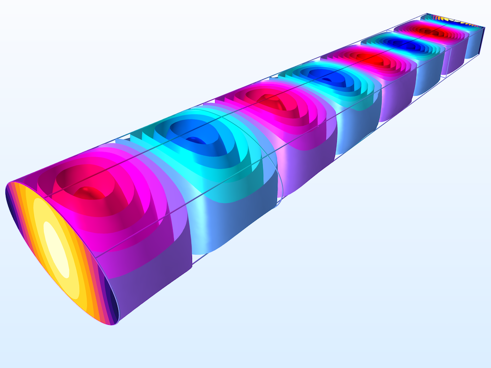
In the waveguide adapter model, the interested frequency ranges between 6.6 GHz and 14.7 GHz, where the TE10 mode is being excited through Port 1. The simulated x-component of the electric field at a frequency of 10 GHz and the S-parameter plot are shown below.

The animation on the left shows the x-component of the propagating electric field on the ports and inside the waveguide adapter at a frequency of 10 GHz. The zy-slice is deformed for visualization purposes. The vertical and horizontal arrows show the direction and intensity of the electric and magnetic field, respectively. On the right, the S11 and S21 parameters (in dB) as a function of the frequency are shown.
The S11 parameter describes the reflections, and the S21 parameter measures the wave that is transmitted through Port 2 when the waveguide adapter is excited at Port 1. Note that:
- It is not possible to excite more than one port at a time if the intention is to compute S-parameters
- We have to add a Boundary Mode Analysis node for each numeric port whether it is excited or not, which results in a study sequence like “Boundary Mode Analysis 1, Boundary Mode Analysis 2,…, Frequency Domain 1,…” under the Study node in the Model Builder
Using Numeric Ports to Analyze Electric Fields as TEM Modes
For a TEM wave or a quasi-TEM wave, the normal component of the electric field to the port boundary (that is, the longitudinal component parallel to the direction of propagation) is negligible. In this case, the numeric port has the option to analyze the field as a TEM mode.
In the Notch Filter Using a Split Ring Resonator model, a split ring resonator is coupled to a microstrip line that is excited and terminated by the numeric TEM port. The circuit acts as a notch (also called a bandstop) filter, which is able to reject a specific signal frequency range. The bandstop frequency is close to 2.4 GHz, as indicated by the S-parameter plot.
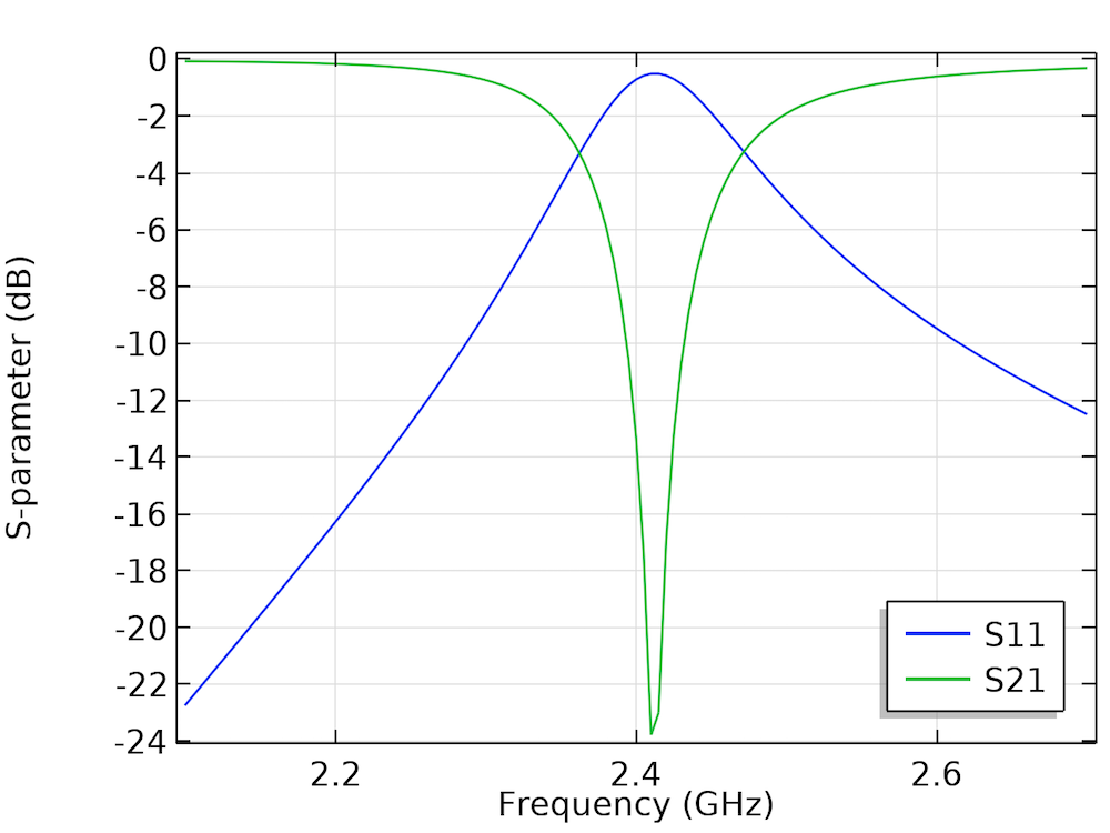
The S11 and S21 parameters (in dB) as a function of the frequency.
It is interesting to visualize the propagation of the electric field at two frequencies; i.e., 2.1 GHz (passband) and 2.4 GHz (stopband).
The z-component of the electric field at 2.1 GHz (left) and 2.4 GHz (right). The xy-slices in both animations are deformed for visualization purposes.
In this model, numeric TEM ports are used to analyze the wave propagation by checking the Analyzed as a TEM field option. When this is done, the port mode field is scaled by the ratio of the calculated and reference impedance. Thus, we have to define the electric and magnetic field integration line under the Port node to calculate the characteristic impedance. The Settings window for Port 1 is shown below. The integration lines for Port 2 are set in a similar way.


The Settings window for the Integration Line for Voltage (left) and Integration Line for Current (right) subfeatures for Port 1 in the notch filter model.
Calculating the Characteristic Impedance Using Mode Analysis
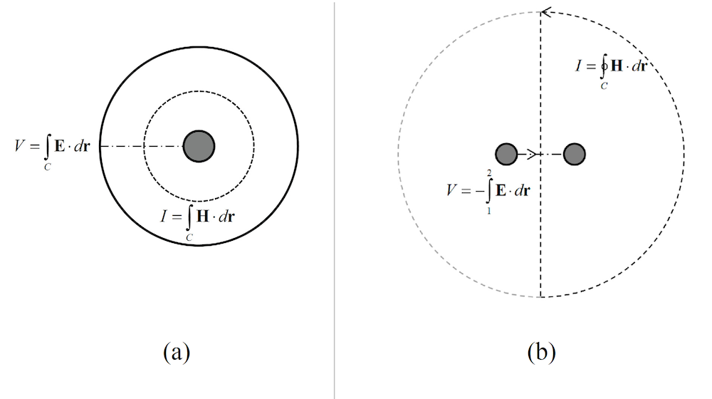
The characteristic impedance of transmission lines can be calculated when the waves propagate in the TEM mode. Two examples available in the Application Gallery are the coaxial cable transmission line and parallel wire transmission line models. The cross sections are simulated in 2D. For both transmission line examples, the voltage (V) is evaluated as a line integral of the electric field that is between conductors. The current (I) is calculated as a line integral of the magnetic field along one of the conductors’ boundaries or any closed contour that divides the area between the conductors into two. The integration lines for the two models are shown in the following figures.
The characteristic impedance is computed as the voltage divided by the current. To do this, we need to define two integration coupling operators, int_E and int_H, for computing the voltage and the current, respectively. The definitions are shown in the table below:
| Name | Expression | Unit | Description |
|---|---|---|---|
| V | int_E( – emw.Ex*t1x – emw.Ey*t1y ) | V | Voltage |
| I | – int_H( emw.Hx*t1x + emw.Hy*t1y ) | A | Current |
| Z | V/I | Ω | Characteristic impedance |
Here, t1x and t1y are the tangential vector components along the integration boundaries (the “1” refers to the boundary dimension). The emw prefix gives the correct physics interface scope for the electric and magnetic field vector components.
For 3D models, boundary mode analysis combined with numeric ports is used to analyze the port boundaries. As described in the above-mentioned 2D models, the characteristic impedance is calculated by computing the ratio between the voltage and current along the edges defined with subfeatures such as Integration Line for Voltage and Integration Line for Current.
Concluding Remarks
This blog post has reviewed the general process for using the Numeric Port feature in the RF Module. With the Numeric type in the port feature, we can compute the desired mode for an arbitrary shape of waveguides and transmission lines as well as excite and terminate the structure. To find the mode field, we have to add a Boundary Mode Analysis study step for each numeric port prior to performing a frequency-domain study to compute the S-parameters, regardless of whether or not the port is excited. Further, we also demonstrated several examples of calculating the characteristic impedance using the Boundary Mode Analysis study combined with the Numeric Port feature when the waves propagate in the TEM mode. The general methods for defining the integration lines when calculating the voltage, current, and characteristic impedance are summarized with two typical transmission line examples.
Next Steps
Learn more about the features and functionality available for analyzing RF models by clicking the button below:
You can also read more about using numeric TEM ports in RF simulations on the COMSOL Blog.


Comments (0)